Open topic with navigation

2D FE Method for Thick-Walled Sections

For arbitrary thick-walled sections a general Two-Dimensional Finite Element approach is applied.

This is the method used automatically in case of multi-material (composite) sections.

Beside thick-walled sections this method can also be applied to thin-walled sections.

As the name indicates, the 2D FE Method discretises the cross-section using two-dimensional elements.

The analysis is split into two separate parts: a Torsion Analysis and a Shear Analysis.

The following paragraphs give more information regarding the determination of the default mesh size and both analysis types.

Default Mesh Size

In case no mesh size is inputted the default mesh size is determined as follows:

1. The cross-section is divided into approximately 250 elements:

With A the area of the cross-section

2. In case the area of the circumscribed rectangle around the cross-section exceeds 10 times the area A the mesh size of the previous step is halved:

This correction accounts for thin-walled sections.

3. The mesh size of the previous step is then rounded using a .5 accuracy. This is the mesh size used for the Torsion Analysis.
   
4. For the Shear Analysis the mesh of the previous step is further refined as follows:

This final step is applied always, also in case a manual input of the mesh size is made.

As with any Finite Element approach, to obtain accurate results the mesh needs to be sufficiently refined.

Torsion Analysis: Prandtl

The Torsion Analysis determines the Torsional constant It, the Warping Constant Iw and the unit torsion stresses.

The analysis is executed according to the Prandtl theory. Within this paragraph the basic principles of the theory are explained.

The Prandtl theory (often referred to as the Membrane or Soap-Film Analogy) is based on the similarity of the torsion stress function equation and the equilibrium equation of a membrane subjected to lateral pressure.

• Consider an opening in an x-y plane which has the same shape as the cross-section to be investigated.
• Cover the opening with a homogeneous membrane.
• The pressure against the membrane causes the membrane to bulge out of plane.
• The lateral displacement z(x,y) of the membrane and the Prandtl torsion stress function φ(x,y) satisfy the same equation in (x,y)

Prandtl Torsion function:

Elastic Membrane function:

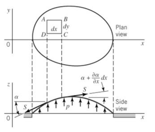
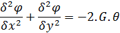
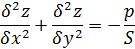
Where z denotes the lateral displacement due to a pressure p and an initial tension S.

The theory concludes with the following:

• Stress components are proportional to the derivatives of the membrane displacement.
• Stresses are proportional to the slope of the membrane.
• The twisting moment is proportional to the volume enclosed by the membrane and x-y plane

Further elaboration and background information regarding the Prandtl theory and 2D FEM analysis can be found in Ref.[1],[7],[8],[9].

The 2D FE Method determines the primary torsion stresses Torsion(Mxp). The values for Torsion(Mxs) will remain zero.

Shear Analysis: Grashof-Jouravski

The Shear Analysis determines the Shear areas Ay & Az and the unit Shear stresses.

The analysis is executed according to the Grashof-Jouravski theory. For background information reference is made to Ref.[10].

The following paragraphs describe the theory for the shear Area Az. The same logic can be written out for Ay.

The theory is generally valid in case the following requirements are met:

• The cross-section symmetrical about the z-axis
• The cross-section is massive, without large holes
• Overall the obtained results are better in case the height is bigger than the width

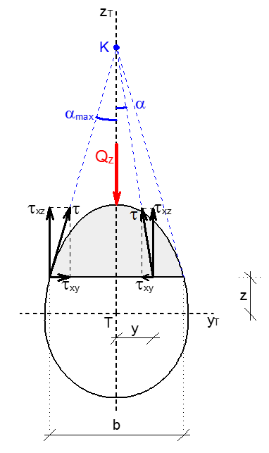
The Shear stresses lead off from the cross-section into one point K.

The area takes on the shear force Q_z.

The value β_z is calculated from the shear stresses in one of the following ways:

1. Only from the vertical components (without influence of )

2. From both components and

In case the cross-section does not meet the requirements of the Grashof-Jouravski theory, the β_z values calculated with the influence of τ_x are absolutely incorrect and often unreal. They should not be used in this case.
Depending on the rate of unrealized conditions, the β_z values which were calculated only from the vertical τ_xcomponent (without influence of τ_x) are real and can be used in this case.
The user should in all cases evaluate if the values determined by the theory are acceptable or not.

In case of multi-material (heterogeneous) cross-sections the calculated shear areas Ay and Az can be used under the following conditions:

• The heterogeneities are symmetrical.
• The heterogeneities do not disturb the Grashof-Jouravski stress theory.
• The heterogeneity is diffused.
• A local heterogeneity consists of less than 10% of the cross-section area.

Openings

As specified, the above theory for shear areas is not valid in case of large openings like for example openings which divide a cross-section into different unconnected parts. A typical example are web openings in steel members.

Specifically for such a case a modified procedure is applied:

In case:

• The cross-section consists of multiple unconnected parts i
• The rotation angle α of the cross-section is 0°

Then the Shear Analysis of the 2D FE Method is used separately for each part i and the shear area Av,i of each part is stored. The final shear area Av of the cross-section is then calculated as the sum of the shear areas of the different parts:

Open topic with navigation