![]()
|
||
|
|
||
To understand better the eigenmodes, the solution of a free vibration system, a SDOF (Single Degree Of Freedom) system is regarded in detail.
Consider the following system:
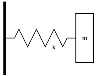
A body of mass m is free to move in one direction. A spring of constant stiffness k, which is fixed at one end, is attached at the other end to the body.
The equation of motion can be written as:

|
(2.1) |
A solution for this differential equation is:

Inserting this in (2.1) gives:

|
(2.2) |
This implies that:

|
(2.3) |
Where ω is called the natural circular frequency.
The natural period T can be written as:

|
(2.4) |
The natural frequency (or eigen frequency) f can be written as:

|
(2.5) |
For a general, MDOF (Multiple Degree Of Freedom) structure, equation (2.1) can be written in matrix notation:

|
(2.6) |
Where:
U is the vector of translations and rotations in nodes,
 is the vector of corresponding accelerations,
K is the stiffness matrix assembled for the static calculation,
M is the mass matrix assembled during the dynamic calculation.
The K-matrix is exactly the same as the stiffness matrix that is used in static computations. In this matrix, proper account can be given to anisotropic material, springs and boundary conditions. For an overview of the possibilities, please consult the manuals which describe the different element types.
From equation (2.6) it is clear that the calculation model created for a static analysis needs to be completed with additional data of masses. In SCIA Engineer, this data is defined and stored in mass groups and mass combinations.
The M-matrix can be computed in different ways. Two classes can be recognised:
-lumped mass matrix, discrete mass in the nodes
-consistent mass matrix, distributed mass on the members
The lumped mass matrix offers considerable advantages with respect to memory usage and computational effort because in this case, the M-matrix is a diagonal matrix. The SCIA Engineer programs will only use lumped mass matrix. By refining the mesh, the lumped converges to the, consistent approach.
The solutions of (2.6) are harmonic functions in time having the following form:

|
(2.7) |
Notice that in this solution a separation of variables is obtained:
The first part, (Φ), is a function of spatial co-ordinates,
The second part, , is a function of time.
When substituting (2.7) in (2.6), an equation is obtained which is known as the Generalised Eigenproblem Equation:

|
(2.8) |
The solution of (2.8) yields as many eigenmodes as there are equations. Each eigenmode consists of 2 parts:
An eigenvalue: value ωi
An eigenvector: vector Φi, which is not fully determined. The deformation shape is known, but the scale factor is unknown.
This scale factor can be chosen in different ways. In SCIA Engineer, as scale factor, a M-orthonormalisation has been implemented. This is shown in the following relation:

|
M-orthonormalisation have following properties:

|
(2.10) |

|
(2.11) |
The algorithm used in the SCIA Engineerprograms to compute the eigenvalues is the well known subspace method. This method is extremely well suited to calculate a relative small amount of eigenvectors. By using this method, N (N is specified by the user) eigenvalues are determined simultaneously. These values will be the lowest eigenvalues if one is using the method straightforwardly.
The program prints each eigenvalue, the radial frequency and the frequency in periods/second. Subsequently, the modal participation factors are given. It is displayed in the calculation protocol of eigenfrequencies. These are defined as:
φjT M {1l}
with :
φjT - the M-normalised eigenvector j
M - the diagonal mass matrix
{1l} - a directional matrix containing a 1 in the indicated direction l and a 0 in other directions
Furthermore, the sum of masses in the analysis is displayed for each global direction X, Y and Z.
The Mass normalised eigenvectors can be displayed both, graphically as in numeric output. The user is allowed to display the mode shapes on the structure. A small tool as available to show it as a animation. For each eigenvector, the deformation of the mesh nodes is listened. The user is allowed to filter the largest amplitude for each global direction. The results are available in the result service “Displacement of nodes”.
The complete list of eigenfequencies is given. For each mode is displayed the frequencies, the velocity, the acceleration and the period. You will find it in the service “Eigen frequencies” in the result menu, which is displayed after a “free vibration” calculation.
To find other related quantities, such as the generalised weight, is easy:
GW = QT W Q
where:
Q - eigenvector with largest amplitude 1
W - weight matrix
From the value of GW, the scale factor to determine φ from Q can be found. If this factor is called a, such that:
Q = φ/a
Then
GW = (1/a)φT W (1/a)φ
= (1/a²)φT gM φgM = W
= g/a²
Similarly, the modal weight can be found:
MW = GW * (participation factor)²
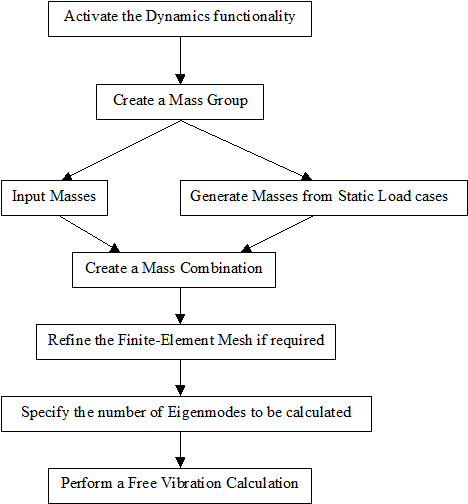
The following diagram shows the required steps to perform a Free Vibration calculation: