Dynamic time-history
Background
SCIA Engineer supports two types of dynamic time history analysis:
- direct time integration; this is the common approach found in literature, where the equilibrium of the structure is explicitly computed in each time step
- modal superposition with time integration; this approach uses a modal decomposition of the structural behaviour; it allows filtering out unwanted high-frequency peaks in the response of the structure and is less computationally intensive than the direct approach
The desired method for time-history analysis can be selected in the solver setup. The modal superposition method is described hereafter. The rest of the settings as well as all the result output features are identical for both methods.
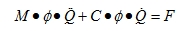
In the modal superposition approach, the eigenmodes are determined first and are used to uncouple the equilibrium equations (1.1) into a set of m uncoupled second order differential equations which are solved one by one by direct time integration. The uncoupling is based on the properties given by equations (2.10) and (2.11). In equation (1.1) a solution for x is assumed to be of the form:

|
(6.1) |
Where φ is the matrix of eigenvectors (n*n) and Q is a vector which is time dependent.
Substitution in equation (1.1) gives:
|
(6.2) |
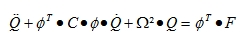
When the equation is pre-multiplied with φT, and equations (2.10) and (2.11) are taken into account, one obtains :
|
(6.1) |
This set of equations is still coupled because of the damping term. If however C-orthogonality is assumed (this means that φT.C.φ reduces to only diagonal terms), then the equations are uncoupled and can be solved separately. The global results are obtained by superposition of the individual results (6.1) is also the exact solution if the assumption of C-orthogonality holds. If however, only a few eigenvectors (m<n) are used in φ instead of all the eigenvectors, then the system of equations and the superposition of the solutions gives a solution x which is an approximation of the exact solution.
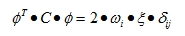
In SCIA Engineer, C-orthogonality is assumed and it is also assumed that all modal damping factors are constant. This means that:
|
(6.1) |
The value of ξ is one of the input data and is called damping factor.
The number of eigenvectors that is taken into account is also specified by the user. This value is equal to the number of eigenvectors computed in the eigenvalue computation.
The method used to solve each uncoupled second order differential equation is the Newmark-method. This method is unconditionally stable but the accuracy depends on the time step. This time step has to be given by the user. However, to help him in his choice, a value determined by the program will be used if the user does not specify a value. This proposed value is computed as:
0.01 T
Where
T- smallest period of all the modes which have to be taken into account
This proposed value guarantees accuracy better than 1% over each period of integration of this highest mode. In most cases, a larger time step can be used because the contribution of this last mode is small.
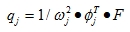
This brings us to the question about the number of modes that should be used. When the time dependent terms on the left hand side of equation (6.3) are neglected, the solution for qj (a term of Q) is:
|
(6.1) |
This indicates that the lowest eigenmodes (ωj small) will contribute more than the highest modes (wj large), if dynamic terms are neglected. This can give a first idea on how many modes to use.
A second criterion is the periodicity of F. Any mode which coincides with the loading frequency should be taken into account.
Modal weight is a third criterion that can be used. If you add all modal weights in a particular direction together and divides this result by 9.81*sum of nodal masses in the same direction, you obtain a value smaller than 1. If this value is close to 1, it means that the higher modes will not contribute anymore. If, on the contrary, the value is smaller than 0.9, one can doubt about the value of a subsequent modal superposition.
Practical use
How to get results
In project data the user selects the functionality “Time history analysis”
The user defined the load case Dead load
The user defines a mass combination
The user defines a load case of type Dynamic with specification General dynamics and setup the parameters of menu “Dynamic load case data” (for example total time 1.5s, step 0.1s, log decrement 5%)
The user de start the linear analysis
The program generated load cases for each time step where the results of that time step are stored.
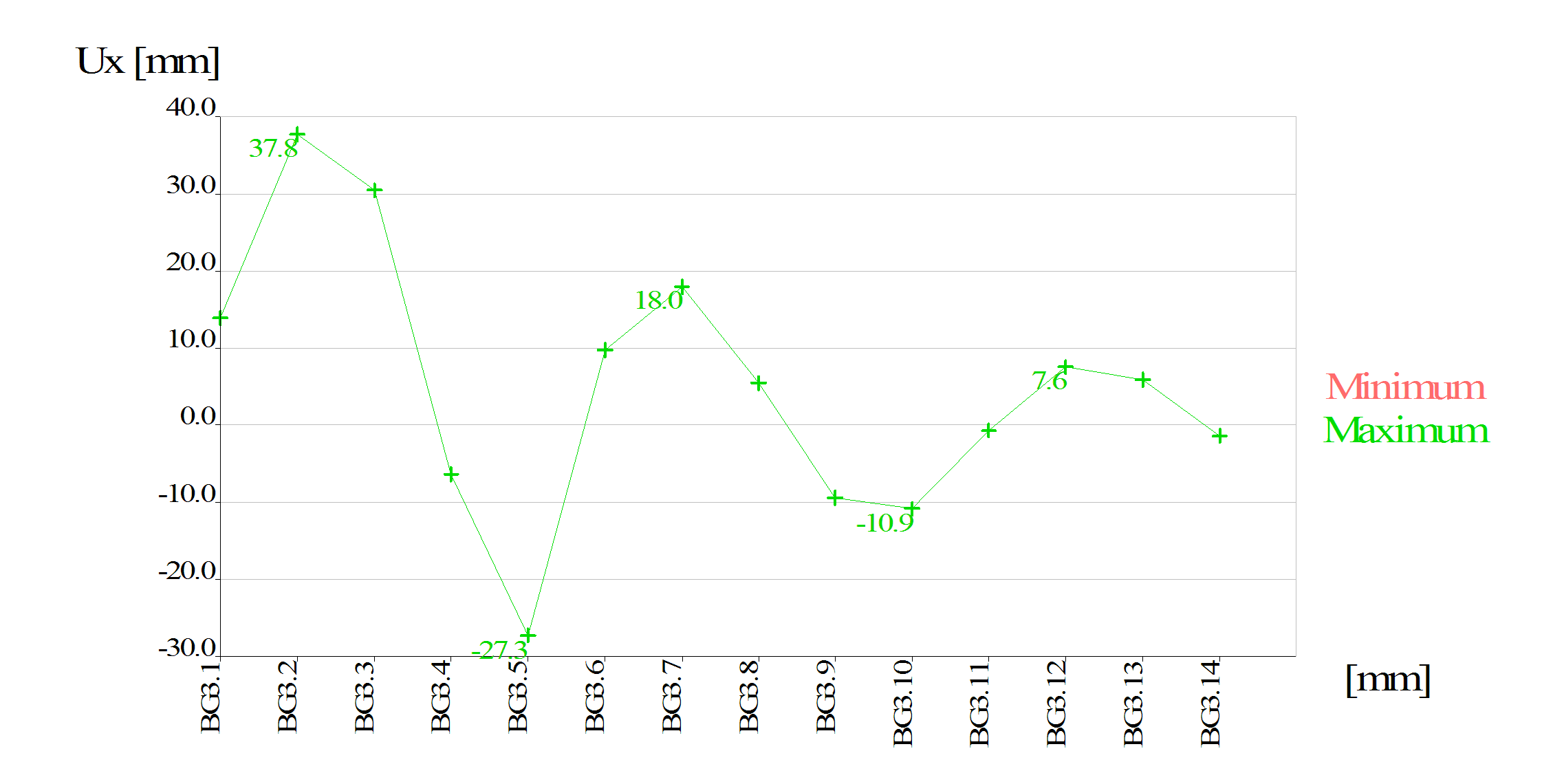
The program generated result class which maces it easy to view the results in graphic form. Bellow an example of the horizontal displacement of a node is displayed for the general dynamic load case BG3.
Remarks
When the user modifies the parameters of the dynamic load case and the starts the calculation again, then the generated load cases are updated.
Then master load case doesn’t contain results.
The generated are stored in an exclusive group and can be used in combination with other load cases
Setup parameters of a general load case
| Total time: | The total time of the dynamic analysis |
| Integration step | Auto, when it is checked, then 1/100 of smallest period is take.When Auto isn’t checked, then the user is allowed to select an integration step value. |
| Output step | Step for generating the load cases. The value need to be smaller or equal at the integration step |
| Log. Decrement | Damping defined as logarithmic decrement |