Seismic loading: Bases of modal analysis
Seismic analysis in SCIA Engineer is based on modal analysis of the structure. This chapter present general theoretical background about modal decomposition of the dynamic behaviour of a model.
SDOF of seismic systems
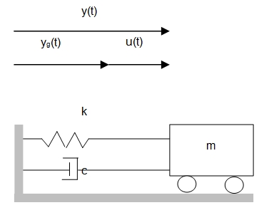
Consider the SDOF system shown in figure bellow which illustrates the displacement of a system that is submitted to a ground motion.
Where:
yg(t) : is the ground displacement,
y(t) : is the total displacement of the mass
u(t) : is the relative displacement of the mass
The total displacement can thus be expressed as follows:

|
(5.1) |
Since yg is assumed to be harmonic, it can be written as:

|
(5.2) |
The equilibrium equation of motion can now be written as:

|
(5.3) |
The inertia force is related to the total displacement (y) of the mass. The damping and spring reactions are related to the relative displacements (u) of the mass.
When (5.1) is substituted in (5.3) the following is obtained:

|
or

|
(5.4) |
This equation is known as the General Seismic Equation of Motion. This equation can be used to illustrate the behaviour of structures that are loaded with a seismic load:
Substituting (5.2) in (5.4) gives the following:

|
This equation can be compared with equation (3.2) of the chapter Harmonic loading. As a conclusion, the ground motion can also be replaced by an external harmonic force with amplitude:

|
When a structure has to be designed to withstand an earthquake, spectral analysis is often used because the earthquake loading is given under the form of a response spectrum. This response spectrum can be either a displacement or a velocity or an acceleration spectrum. The relation of an earthquake given by an acceleration time history and the corresponding spectrum is given by:

|
(5.5) |
With:
 : Ground acceleration in function of time
 : Damping factor
 : The period
The integral between the square brackets is known as the Duhamel integral. This integral is the solution of the differential equation (5.4).
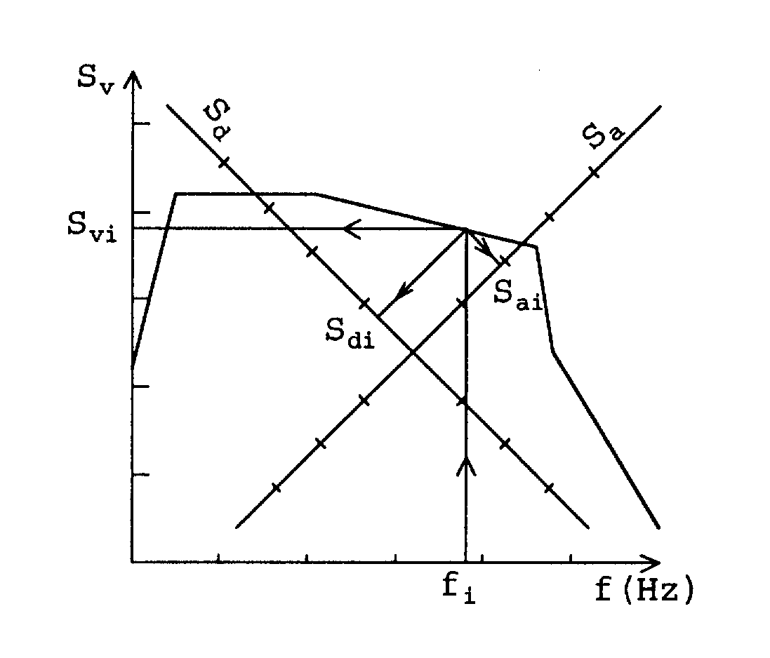
Instead of Sd (displacement response spectrum), Sv (velocity response spectrum) or Sa (acceleration response spectrum) can be used. These spectra are related by ω :

|
(5.6) |
The three spectra are normally given on the same figure, using different scale-axes. (See picture of spectral density bellow)
MDOF of a seismic system
For MDOF (Multiple Degree Of Freedom) systems, equation (5.4) can be written in matrix notation as a set of coupled differential equations:

|
(5.7) |
The matrix {1} is used to indicate the direction of the earthquake. For a two-dimensional structure (three degrees of freedom) with an earthquake that acts in the x-direction, the matrix is a sequence like {1,0,0,1,0,0,1,0,0,…}
The resulting set of coupled differential equations is reduced to a set of uncoupled differential equation by a transformation  , where Z is a subset of Φ (the eigenvectors) and Q is a vector, which is time-dependent.

|
or

|
This can be simplified to a set of uncoupled differential equations:

|
(5.8) |
Where C* is a diagonal matrix containing terms like  .
.
Each equation j has a solution of the form:

|
(5.9) |
To obtain the maximum displacements, the displacement response spectrum Sd of equation (5.5) can be substituted:

|
(5.10) |
And:

|
(5.11a) |
Or:

|
(5.11) |
Where  is known as the modal participation factor.
One obtains in each node a value of (Uj)max, j=1,m (m<n). The maximal global displacement is the sum of the absolute values of the displacements, assuming that the peak value of all considered modes occurs at the same moment. As that assumption is unrealistic and very conservative, often, the RMS (root mean square) is used as maximal displacement:

|
(5.12) |
SCIA Engineer supports 3 superposition methods:
SRSS (Square Root of Sum of Squares)
CQC (Complete Quadratic Combination)
MAX (max method)
A detailed description is given in the next chapter, "Seismic loading: Modal superposition".