Nonlinear calculation
Definition, application
In general, when modelling structures, a linear approach is followed. It can however be that certain parts of the structure do not behave linearly. Examples include supports or members which only act in compression or tension. This is where non-linear analysis is required. Another example is when performing structural analysis following the latest codes (i.e. Eurocode 3). When performing manual calculations, in most cases a linear 1st Order analysis is carried out. However, the assumptions of such analysis are not always valid and the codes then advise the use of 2nd Order analysis, imperfections, etc. Scia Engineer contains specialized modules covering non-linear related issues.
The main difference between a linear and non-linear calculation is that the non-linear calculation gives such results of deflections and internal forces for which equilibrium conditions are satisfied on a deformed structure. The user should think beforehand whether the load applied on the structure would lead to such a state of deformation that affects the resultant internal forces and deflections. If the user thinks so, they should use the non-linear calculation at least for one selected load and compare the results with those for linear calculation. Thus, the user can evaluate the effect on non-linearity on behaviour of the structure.
Nonlinear calculation it is an iterative process. This process is defined by two basic settings: “Number of increments” and “Number of iterations” in every increment. It means load applied on structure is divided into increments and in every increments there is limit of iteration of calculation. So it is clear, that calculation can take a long time if solution is complicated or structure is very big. In solver we have implemented 4 basic types of calculation methods: Newton-Raphson; Modified Newton-Raphson method ; Picard method; Picard and newton Raphson. Every method has some advantages and disadvantages, but according user choice of nonlinearities in list in project data SEN automatically set some defaults, which should be the best choice for most of structures.
The non-linear calculation in SCIA Engineer is based on the following assumptions:
-
equilibrium conditions are satisfied for deformed shape of a structure,
-
effect of axial forces on flexural stiffness of beams is taken into account as well,
-
non-linear supports are taken into consideration,
-
material of the structure is considered as linearly elastic.
Basic settings for non-linear calculations
In project data dialog – functionality tab – list of possible nonlinear functionality dependent on modules in license.
After check, new items and settings will appear in different parts of GUI SEN.
As a basic activation of nonlinear calculation, it is necessary to do two things:
1) Checked functionality in project data dialog
2) Create " Non-linear combinations"
If these two things are done, in solver setup there are new settings for nonlinear calculation and in calculation dialog there is active possibility to calculate “nonlinear analysis”.
Selection of nonlinear functionalities
If any kind of non-linearity should be taken into account in a project, it is necessary to select appropriate option (or options) in the Project data dialogue.
The possible Functionalities related to non-linearity are listed if the main option"Functionality - Nonlinearity" is chosen.
Solver setup
All calculation settings are located in "Solver settings" . There is a part with partameters only for non-linear calculation and it enables to user to define additional options described in table below.
|
Geometrical nonlinearity |
This option is available only for functionality "Geometrical nonlinearity" in project. This is a combobox with two possibilities, where user can define geometical nonlinearity according "2nd order" or "3rd order". The "2nd order" is the exact solution of differential equations according Thimoshenko theory. This settings is suitable for most nonlinear behavior of buildings and it is default settings. Default iterative method of calculation is Picard method. The "3rd order" it is an iterative solution mostly for projects with membranes and cables, where there may be large deformations. Default iterative method of calculation is Newton-Raphson method. |
|
Method of calculation |
This item shows which iterative method will be use by solver for this nonlinear calculation. There are four types of method: Newton-Raphson, Modified Newton-Raphson, Picard and Picard and newton Raphson. User can edit this item only if geometrical nonlinearity is set as 3rd order. |
|
Number of increments |
This parameter is applied for both Newton-Raphson and Timoshenko method only. The values for individual methods are independent and remembered by the programme. Therefore, if you adjust 1 increment for Timoshenko method and four increments for Newton-Raphson method, this parameter will change every time you swap from one method to the other. Usually, one increment gives sufficient results. If deformation is large, the calculation issues a warning and the number of increments can be increased. The greater the value is, the longer it takes to complete the calculation. |
|
Maximum iterations |
Specifies the number of iterations for the non-linear calculation. This value is taken into account only for the Newton-Raphson method. The termination of calculation is controlled by means of convergence accuracy or by means of the given maximal number of iterations. If the limit is reached, the calculation is stopped. If this happens, it is up to the user to evaluate the obtained results and decide whether (i) the maximum number of iteration must be increased or whether (ii) the results may be accepted. For example, if the solution oscillates, the increased number of iterations won’t help. |
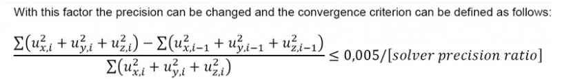
| Solver precision ratio |
Coefficient that affects the tolerances used during non-linear analysis for convergence checks. Tolerance values are divided by that coefficient. 1 means that the nominal tolerance values are used. A coefficient value higher than 1 means that the tolerances will be smaller, hence the calculation will be more accurate. A coefficient value lower than 1 means that the tolerances will be larger, hence the convergence will be achieved more easily. In some case of heavy non-linearity (e.g. cable or membrane structures), it might be necessary to use less strict convergence criteria (e.g. ratio = 0.1) to allow for proper convergence of the analysis. Note that even with a ratio = 0.1, the convergence criteria remain very tight.
|
| Solver robustness ratio | This parameter affects the damping (speed of change) of the stiffness and internal forces of non-linear hinges, supports, members. It is not possible to exactly describe it, because it is always a little different in different cases and types. It influences the convergence of nonlinear calculation with local nonlinearities on 1D members, hinges and with nonlinear surface support independently on selected method of calculation. O a high value of this parameter ensures a more stable but slower convergence of the calculation. It can help in case of sensitive nonlinear analysis where convergence is problematic. |
|
Plastic hinge code |
If this option is ON, the non-linear calculation takes account of plastic hinges. It is possible to select the required national standard that will be used to reduce limit moments. If no standard is selected, no reduction is performed. |
|
Allow compression in membrane members |
If this checkbox is ON, the compression in membran elements is taken into account. |
Limits of the calculation
|
Total number of nodes and finite elements |
unlimited |
|
Total number of non-linear combinations |
1000 |
|
Maximal number of iterations (in one increment) |
1000 |
|
Maximal number of increments |
500 |
Calculation protocol
After nonlinear analysis it is possible to look at " Calculation protocol - Nonlinear" where all basic info about it are stored.
Note: Static non-linear calculation can ONLY be performed after the static calculation of the same project has been carried out successfully. In other words, non-linear calculation is a two-step procedure: (i) linear calculation must be completed, (ii) non-linear calculation can be started.