1D FE Method for Thin-Walled Sections
For thin-walled sections (open or closed or a combination of both) a general One-Dimensional Finite Element approach is applied. For a detailed background regarding this method including calculation examples reference is made to Ref.[1].
Centerline
The centerline representation of a cross-section concerns an idealized 'skeleton' profile which shows the general element geometry and connectivity Ref.[13].
This representation suggests that all the 'linkages' in the section will traverse along the line of mid-thickness of each component regardless of their thickness.
Generation
The centerline is generated in two steps. In the first step, the centerline of each separate thin-walled part is generated at the line of mid-thickness:
In the second step, when two thin-walled parts are touching, the centerlines are extended until they intersect. These extensions form additional centerline elements.
The centerline extensions have a thickness equal to the thickness of the centerline element from which they were extended. The maximal length of the extension between two centerline elements 1 and 2 is 0,5 * (t1 + t2) with t1 the thickness of centerline element 1 and t2 the thickness of centerline element 2. When the distance of the extension would exceed this limit, no intersection is made i.e. the thin-walled parts are seen as not connecting.
Thickness
Each centerline element has a constant thickness. The centerline is thus split into multiple parts in case there is a difference in thickness.
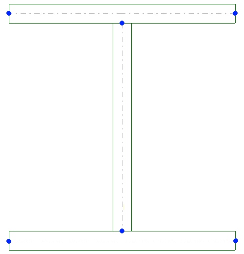
Fictive elements
In case parallel thin-walled parts are touching in an asymmetric way i.e. not directly through their mid-line, a "fictive" element is added to ensure connectivity between the different parts.
This fictive element is used purely for 'linkage' purposes and is given a thickness which is negligible compared to other 'normal' centerline elements (1e-10 mm).
In very special cases the generation of fictive elements can lead to unrealistic results. A typical example concerns a closed pair section formed out of two cold-formed C-sections. In this case, the fictive elements are located on the outer centerline of the closed shape. Due to their negligible thickness this will lead to an unrealistic torsional constant. For such cases the 2D FE Method should be applied instead.
Fused elements
Parallel thin-walled parts which are joined by for example welds are replaced by a single centerline element with a thickness equal to the resulting thickness sum. This simulates that these parts have been 'fused' together into one idealized combined part.
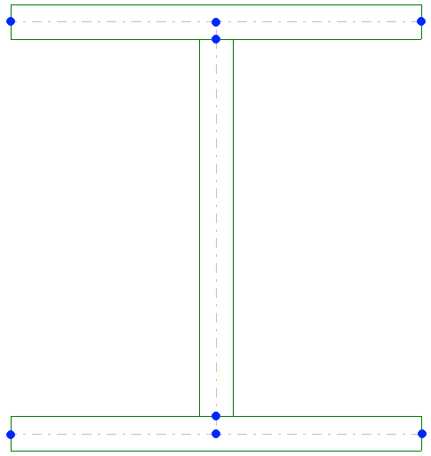
The following example illustrates this in case of an I-section which is welded to the web of a larger I-section:
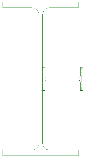
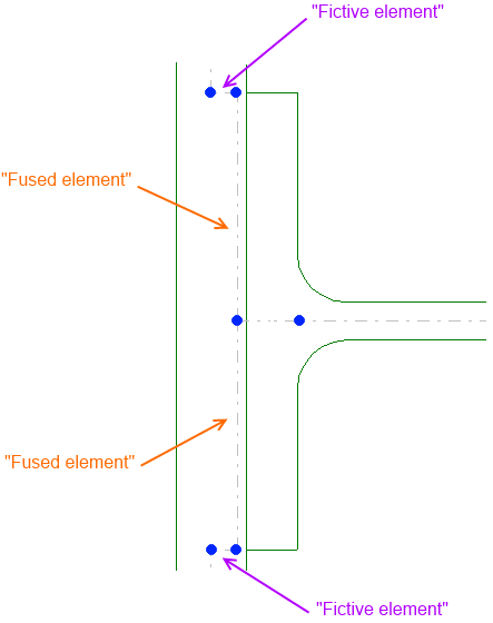
At the position where the flange of the small section and the web of the large section are connected together, a single "Fused" centerline element is generated with thickness equal to the sum of both element thicknesses. In order to connect this element to the rest of the web of the larger I-section, "Fictive" elements are used.
In this example, the "Fused" element in turn is split in two due to the intersection with the extended web centerline of the smaller I-section.
Curved elements
In case a general thin-walled cross-section is inputted it is possible to define curved elements. For the centerline generation curved elements are not accounted for and replaced by straight elements as follows:
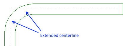
- In case the angle between straight parts (connected to a curved part) is <= 135° then the intersection is made between the extension of the centerlines of the straight parts.
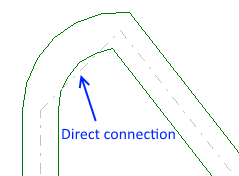
- In case the angle between straight parts (connected to a curved part)is >135° then a simplification is used since no intersection can be found or the intersection is far away from the rounding position. In this case the straight parts are directly connected.
Calculation Procedure
Based on the centerline the cross-section is discretised into nodes and elements as schematised on the following picture:
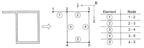
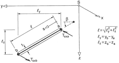
Each element is defined with a begin node a, an end node b and a constant thickness t.
The Finite Element analysis is carried out using the following steps:
Step 1: Calculation of the warping ordinate 
Equation system (boundary condition:  ):
): 
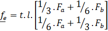
Element matrices:
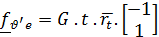
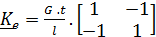 ,
, 
with:
 for D = S
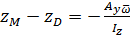
Step 2: Position of the shear centre and standardisation of the warping ordinate:
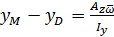 ,
, 


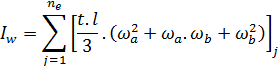
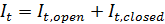
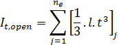
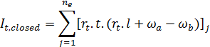
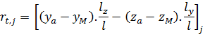
Step 3: Calculation of the cross-section properties Iw and It
Step 4: Calculation of shear deformations due to shear forces and secondary torsion:
Equation system (boundary condition: ui = 0 ): 
with:
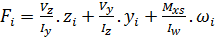
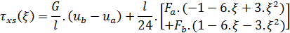
Step 5: Calculation of shear stresses:
Shear stresses due to primary torsion:
linearly via t with: 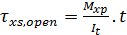
constantly via t: 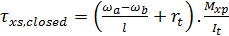
The unit (primary) torsion stress per fibre is then calculated as the superposition of the absolute values of  and
and  .
.
Shear stresses due to shear forces and secondary torsion:
The above procedure is given here for informative reasons. For a full description of all abbreviations used in this procedure as well as background information and worked out examples, reference is made to Ref.[1].
The main advantage of this method is that it can be used for both open and closed thin-walled sections or combinations of both (sections with openings and outstands). The method is however only valid for sections with a continuous centerline i.e. where all parts are connected by one continuous line.
Additional Step: Calculation of unit warping stress
The above calculation procedure is extended with the calculation of the unit warping stress per fibre:
 in which Mw is taken as a unit bimoment.
In case of multiple unconnected parts (like a pair section composed out of two thin-walled sections which do not touch each other) the 1D FE Method cannot be applied since there is no continuous centerline. In such cases the 2D FE Method should be applied.
Fibre Mapping
The results calculated using the 1D FE Method as outlined in the previous paragraph are determined on the centerline. These results need to be 'mapped' to the fibres of the cross-section which will then be used in the stress checks etc.
Standard case
The fibre mapping is done in two steps. In the first step, for a given fibre, the normal projection of the fibre to each centerline in the cross-section is made. Only centerlines for which this length of the normal line is smaller than the thickness of the centerline element are kept.
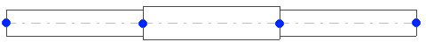
This principle is illustrated on the picture below:
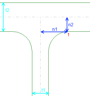
For fibre 1 the normal line to centerlines 1 and 2 is made.
The length n1 of the normal line to centerline 1 exceeds the thickness t1 of this centerline. Therefore this centerline is not kept.
The length n2 of the normal line to centerline 2 is smaller than the thickness t2 of this centerline. Therefore this centerline is kept. In other words, the fibre is found to be more closely positioned to centerline 2 than to centerline 1 and thus the fibre will receive results from centerline 2.
In the second step, for the centerlines which are kept, the result values are determined at the points of projection of the fibre. Of those results, the maximal value is stored as the result value for the fibre.
Centerline extension
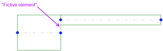
In case for a given fibre no centerline is found, a special procedure is executed. This is a typical result in case of the corner point of an L-section:
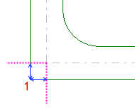
In the above picture, fibre 1 is outside of any centerline so no normal line can be determined. In this case, all centerlines are extended at the begin and at the end with 20% of their length.
The centerline results on the extension at the begin are taken equal to the result at the begin point, the centerline results on the extension at the end are taken equal to the result at the end point of the centerline.
After this extension again the normal lines and final fibre results are being determined as in the previous procedure.
In case, even after this extension, a fibre is still located outside of any centerline, it does not receive any result mapping.