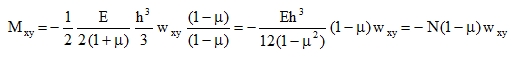
Shape orthotropy of plates

Main principles of the transformation into physical orthotropy

Certain bridge, floor, foundation and other structures are similar to plates in terms of the hypothesis (11), i.e. their total “thickness” h is small in comparison with plan-dimensions L. On the other hand, they represent a body of a more general shape, e.g. ribbed plates, hollow core slabs, plates with both weak and stiff reinforcement, e.g. with I-beams embedded in the concrete, corrugated plates, double-layer braced plates, etc. Only occasionally is the total flexural stiffness of such shapes identical in both (i) longitudinal x-direction and (ii) transverse y-direction. Usually, the stiffness in the two directions can differ even by a factor of ten. This is not due to different modulus E₁ and E₂, but due to a varying section in planes x=constant. It is therefore the shape (not physical) orthotropy of the plate in terms of shape or technical orthotropy. Global behaviour of such plates (without a detailed stress analysis in the vicinity of statically, geometrically or physically singular points and without other irregularities due to the real shape of the body) can be analysed by means of methods and programs developed for physically orthotropic plates, as long as the following assumptions are taken into account:

Displacement components u, v, w (3) must be unequivocally derivable from the plate deflection surface w (or from the three functions (2) in case of plates with the effect of shear taken into account) across the whole analysed body, which means also its deformation ε and stress σ components, or the internal forces acting in the section across any part of the body. This requires establishment of suitable geometrical hypotheses, such as (4), verified in terms of accurateness through various reasoning, experiments, practical experience, etc.

Based on the hypotheses (a), the following must be unequivocally specified for every type of shape orthotropy in plates:

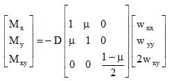
b1) INPUT: Constants D_ik in the matrix of physical constants D for physically orthotropic plate that is going to substitute the analysed plate in the calculation.

OUTPUT: Further utilisation of outputs of internal forces in the substitute physically orthotropic plate for the needs of design and checking of the analysed plate with shape orthotropy, i.e. what internal forces or what stresses arise in the analysed plate.

An accurate analysis of meeting the assumptions (a) and accurateness or technical applicability of results would require a comparison with the exact three-dimensional solution of a real structure at least in several characteristic or limit states, or with reliable experiments and tests. This is available only for certain examples, e.g. for steel ribbed plates, etc. Then, more precise data about the composition of the slab section appear in the input (b1). Mostly however, such analysis can not be performed and only an approximate method can be used for the comparison, e.g. for box-section plates, which, however, is not a proof, as the variation from the exact solution is not known. In view of numerous factors that influence the properties of civil engineering structures, some well-tried formulas – extended by up-to-date knowledge about, in particular, torsional stiffness – can be accepted for the approximate calculations.

Simple types of orthotropic plates

Energetic equivalence of sectional characteristics

In paragraph 6.2 we will discuss plates in which the effect of transverse shear can be neglected and in which the classical Kirchhof hypothesis (4) is satisfied within the whole range. Practically speaking, these are common, not-too-thick plates that are ribbed, corrugated or stiffened in two directions x ^ y identical with the selected direction of coordinates (e.g. [1], p.37, Fig.9).

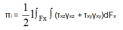
The principle of potential energy equivalence of internal forces in the real and substitute body must be observed in the transformation into a physically orthotropic plate, i.e. in the calculation of constants D_ik in the stiffness matrix (16). For the plates in question, it is the following formula

(35)

which is the integral of the products that represent only work of moments (similarly to a slim beam subjected to bending and torsion) on curvatures that can be, for small deflections w, expressed by second derivatives. In the calculation of the substitute plate by means of the finite element method, the second mixed derivative will be continuous everywhere (or at least everywhere with the exception of shapes with zero surface area) and the following condition of equivalence is met

wxy = wyx .

(36)

Similarly, the theorem of reciprocity of torsional moments will be valid in the substitute plate:

Mxy = Myx

(37)

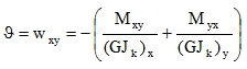
and thus (29) can be simplified to:

(38)

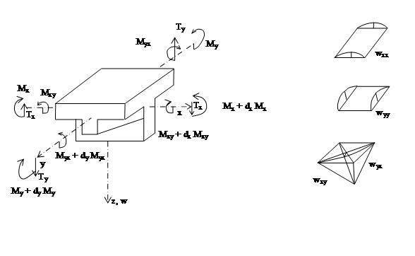
Fig.  2

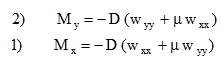
The positive direction of all quantities is shown in Fig. 2. The comparative level (Π_i = 0) is the primary non-deformed shape. Π_i is always positive.

Let us have a system of two beam skeletons that are parallel to x- and y- axes and have flexural stiffness (E’J)_x, (E’J)_y, torsional stiffness (GJ_k)_x, (GJ_k)_y, flexural curvature κ_x = w_xx,, κ_y = w_yy  and relative twisting ϑ_x, ϑ_y. The potential energy of bending and torsional moments of such a system is

(39)

Comparing (39) with (35), we can get – only formally at the moment – the following formulas for plate strips of unit width d_x = 1 or d_y = 1:

(40)

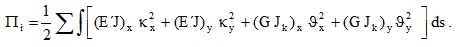
As the transverse contraction and elongation of element sections cannot occur freely in a compact plate (Fig. 3),

Fig.  3

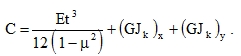
the plate strips are rather stiffer in bending than the beams. This can be included into the modulus of elasticity, and thus e.g. in the case of an isotropic plate we have the module

(41)

which follows from the exact relation between σ and ε. In addition, it can be seen in Fig. 3 that the transverse contraction of the section is prevented in plates by certain transverse moments M’. E.g., the transverse moments occurring in isotropic plates subjected to bending moment M_y and deformed to a cylindrical surface w(y) are

M´ = Mx = μ My

(42)

and similarly, in plates subjected to bending moment M_x and bent to the surface w(x) we have:

M´ = My = μ Mx ,

(43)

This effect vanishes in materials without transverse contraction (μ = 0).

Let us examine the consequences of formal equations (40) to (43) in isotropic plates with the thickness h << 1, so that

(44)

Let us employ the well-known relation for shear modulus

(45)

and let us name the known plate-constant as

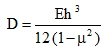
(46)

We get formulas defining the relation between moments and curvature

(47)

that are in full compliance with formulas derived from the hypothesis (4). In addition, using Fig. 4, let us consider that the total twisting ϑ (more precisely the torsional curvature) of the plate element is influenced by both pairs of torsional moments, so that

(48)

Fig. 4

In plates the continuous mixed derivative w_xy = w_yx = ϑ (see also Fig. 2, the element is deformed into a warped line surface of a hyperbolic paraboloid type 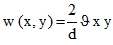in local coordinates x, y with the origin in the centre of the element, so that in the corners 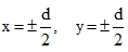we get w = ± w₀. A general formula then follows from (40)

(49)

and in the case of isotropic plates it is

(50)

 

After substitution from (44) and (45), multiplication by one in the form of and use of

(1+μ) (1-μ) = (1-μ²) we obtain

(51)

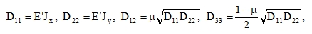
which is the same formula that can be derived by an accurate procedure (integration of τ_xy) from hypothesis (4). Therefore, the beam-based theorization about physical constants of a plate leads to the correct stiffness matrix D of an isotropic plate. Using (16) or (33), (47) and (51), we can write it in the form usual in FEM:

(52)

It can be therefore expected that such a theorization will not be principally (i.e. as far as equilibrium and continuity conditions are considered) defective even in simple plates with shape orthotropy, which is also supported by the existing experience obtained in experiments and in real practice.

Bending and torsional moments

The dimension of these quantities is force, or more clearly, force × length per unit width of a plate section. Using the main SI units, it is N (Newton) or Nm/m (Newton meter per 1 meter of width).

Conversion to previously used units:

1 kp =  9,80665 N = 10 N

1 Mp=10 ⁴N = 10 kN

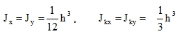
All sectional characteristics J_x, J_y, J_kx, J_ky must be calculated either (i) for a unit width of a section or (ii) for another width of the section ‘b’, e.g. for the distance between ribs or the size of the finite element and then the result must be divided by this ‘b’. The dimension of J is therefore m³.

Plates without transverse contraction

This group includes practically all ribbed plates with open ribs (not hollow core slabs), because the flexural stiffness of such plates is derived mainly from ribs that do not influence each other in transverse direction as there is no continuous contraction in this direction. The value termed as “effective value of μ” is very small (e.g. 0.02) also in reinforced concrete plates with thin ribs, especially after the formation of cracks in the tensile concrete, and calculations of such plates for μ = 0 are accurate. The matrix of physical constants is diagonal as D₁₂ = D₂₁ = 0, see (28). What remains is to determine D₁₁, D₂₂, and D₃₃.

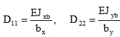
The first two bending constants are quite clear and they can be calculated using (40) from

D11 = (EJ)x, D22 = (EJ)y, [Nm].

(53)

The formulas include also possible diverseness E_x ≠ E_y [Nm^-2]. J_x, J_z [m³] are related to the unit width of plate sections in planes x = constant and y = constant. For the most common situation of E_x = E_y = E and for the calculation of J_xb, J_yb [m⁴] for ribs with an effective width of the plate b_x, b_y we have

(54)

If the plate of the height h is ribbed only in its x-direction, then

(55)

For the needs of this calculation, in common concrete plates with ribs in both x- and y- direction, the full distance shown in Fig. 5a can be taken as the effective width b_x, b_y.

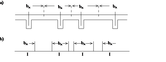
Fig.  5

Only for thin plates, e.g. steel orthotropic deck slabs, the reduction of b_x, b_y according to technical standards is more significant (Fig. 5b). It is however necessary to considered the real loading conditions of the plate and other circumstances and not only apply the formula given in the standard, as it is valid for stress rather than for the substitute flexural stiffness. When b_x, b_y are uncertain, we recommend a consultation with the author of this guide.

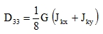
The third constant, torsional D₃₃, is more problematic, but in most situation we can get satisfactory result using the formula that follows from (24) for μ = 0.

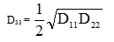
(56)

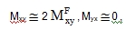
For isotropy and μ = 0, this formula transforms into the correct value of 1/2 D, see (52). This is then represented by one torsional moment M^F_xy = M^F_yx of the substitute physically orthotropic slab.

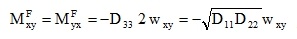
(57)

The equality M^F_xy = M^F_yx follows from the theorem of reciprocity of shear stresses τ_xy = τ_yx (Fig. 6a) that must be valid on the vertical edge of the plate element also in plates with shape orthotropy, but that does not imply the equality of torsional moments, which clearly follows from Fig. 6b. Torsional moments can be obtained by the integration of the shear stress flow over the section through planes x=constant and y=constant:

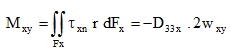
	(58)
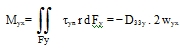
	(59)

In order to apply formulas (58 and 59) accurately, we would have to know the exact distribution of shear flow over the sections of the given plate with shape orthotropy. It is quite a difficult three-dimensional problem that would require rather challenging application of the finite element method. Therefore, let us perform first an approximate technical calculation based on the estimate of torsional stiffness strips, like beams in a grate, without continuous dependencies. As w_xy is a continuous function in plates, we have

w_xy = w_yx (Fig. 6c) and the comparative beams have the same relative twisting angle, and thus the ratio of moments (58) and (59) is

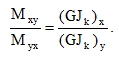
(60)

Let us define a sum-relation between moment (57) and moments (58), (59) that is not in contrast with the isotropy. If we compare the formulas for energy (35) and (38) where there is a continuous mixed derivation of the function w, in which w_xy = w_yx, it follows:

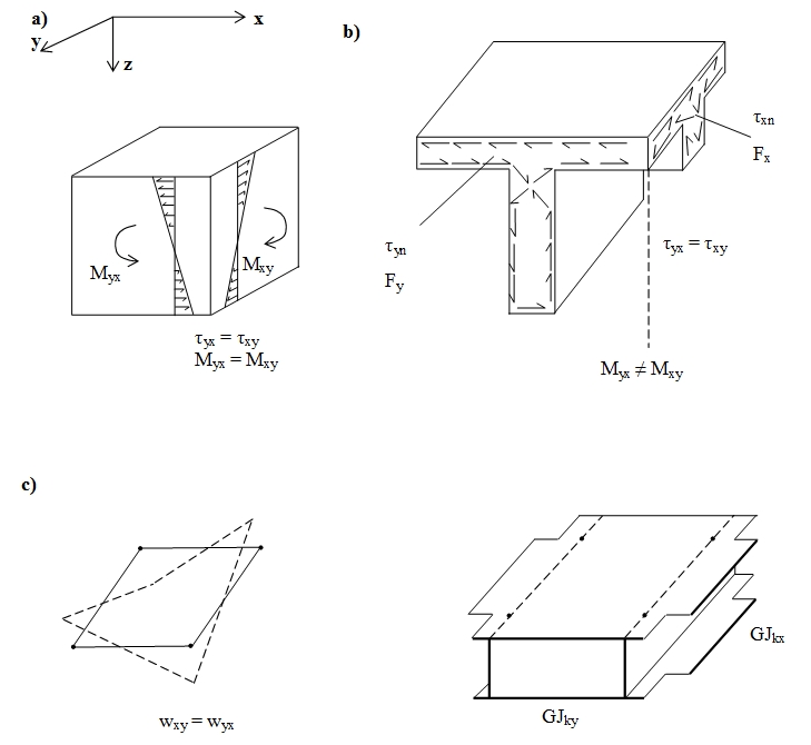
Fig.  6

(61)

This leads us to the following values:

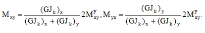
(62)

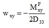
Substituting (62) into the formula (49) we get

Comparing with the formula (57)

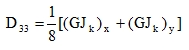
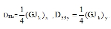
we obtain the formula that will be used to calculate the input value D₃₃, i.e. the torsional stiffness of the substitute physically orthotropic plate.

(63)

Quantities J_x [m³] are related to a unit width of the section. Usually, they are calculated for another suitable width (beam-like section) b, so that J_k = J_kb [m⁴]: b [m].

The drawback of this approach is that a pure Saint-Venant torsion is prevented in the plate in the x- and y- direction, as:

the surface shear stress is not zero (τ ≠ 0 on vertical sides of the surfaces ) over the whole surface of these strips,

free warping is prevented in these strips.

The deviation is not too large in rather thin plates with rather thick ribs. Under different configuration this approach can be applied if everywhere │M_xy │‹ │M_x ,M_y│. If we calculate quantities J_k from the accurate shear flow (58) and (59), the approach will be always acceptable. Exceptions, such as plates with encased I-beam etc, should be consulted.

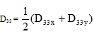
Approximate calculations of common structures can be performed with D₃₃ determined from the formula (56) that does not require identification of torsional stiffnesses. It can be proved that both the formula (56) and the future formula (72) for plates with transverse contraction are in the case of isotropic plates identical with the formula (63), see the reasoning in paragraph 6.2.1 following the formula (44). It generally follows from (61) that

(63a)

and in our simplification we have

Let us remind that the first subscript of τ and M always denotes the area (section x = constant) on which τ or M acts. The moment M_xy thus shortens the plate strips parallel to the x-axis, and the moment M_yx the strips parallel to the y-axis. See also Fig. 4 where the positive direction of these moments can be clearly seen.

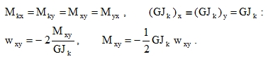
Two special situations for formulas (62):

a) A plate with the same torsional stiffness in the x-direction and y-direction, i.e. J_kx=J_ky and M_xy= M_yx= M^F_xy is the printed value of the torsional moment.

b) A plate with a predominant torsional stiffness in one direction, caused e.g. by thick ribs that are rigid in torsion in one direction – let us mark it x. It is characterised by a strong inequality J_ky‹‹ J_kx. In such a plate the formulas (61) and (63) give

and thus the torsional moment in the x-direction is the double of the printed moment and it is zero in the y-direction.

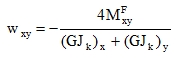
The real value is between the limits of type (a) and (b). If we deal with what is called design moments represented in outputs by values

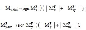
(64)

it must be considered that (the superscript F still means the physically orthotropic plate for which the whole calculation is done), but is only a formal value. The application of values (64) is therefore useful for situations approaching the limit of type (a). Otherwise, it would be reasonable to use a correction in the meaning of the formulas (61) or (63).

Plates with transverse contraction

Coefficients of transverse contraction in plates with shape orthotropy can be, following from (16) to (18), assigned the following visual meaning (Fig. 7):

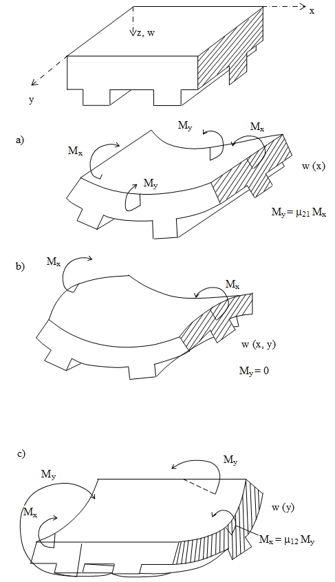
Fig.  7

Let us deform the plate element as in Fig. 7a into the shape corresponding to a cylindrical surface w(x) with a constant curvature w_xx. Then w_yy = 0 and, according to (16), the following moments are necessary to cause such deformation:

Mx = -D11wxx ,  My = -D21wxx = μ21Mx.

(65)

If we subject the element only to moment M_x, it would lead to a state shown in Fig. 7b, because the following condition follows from the second line of (16) with M_y = 0:

D21wxx+D22wyy = 0 ,

and therefore, the element would be distorted also in the y-direction with the curvature w_yy = -D₂₁w_xx / D₂₂ = -μ₁₂w_xx. To produce the same curvature w_xx, smaller moment would be sufficient:

Mx =  -D11(1-μ21μ12) wxx.

Similarly, the following moments are necessary to produce a cylindrical deflection w(y) of the element in the y-direction (Fig. 7c):

My = -D22wyy ,  Mx = -D12wyy = μ12My.

(66)

If the load is formed only by moments M_y, i.e. if M_x = 0, it leads, according to the first line of (16), to a non-zero curvature w_xx = -D₁₂w_yy/ D₁₁ = -μ₂₁w_yy. To produce the same w_yy, a smaller moment is necessary:

My = -D22(1-μ12μ21) wyy.

Therefore, for plates with shape orthotropy we can introduce the following definition of the coefficients of transverse contraction:

The coefficient μ₂₁ is numerically equal to the moment M_y that must be applied to y=constant-edges of the element that is subjected to moment M_x = 1 on edges where x=constant, in order to bend the element into a cylindrical surface w(x). Similarly, the coefficient μ₁₂ is the value of M_x on x=constant-edges of the element subjected to moment M_y = 1 on edges where y= constant and bent to a cylindrical surface w(y). It can be easily verified that in the case of physically orthotropic plates this definition is equivalent to the original definition (8) and in the case of isotropic plates it results in the known relation μ₁₂ = μ₂₁ = μ . At the same time, with this definition it is clear that if the structure resembles a strong grate with a thin plate, it is practically true that μ₁₂ = μ₂₁ =0 and formulas from paragraph 6.2.2.1 are applicable.

The Maxwell-Betti theorem for plates with shape orthotropy:

If a plate element is subjected only to moment M_x = 1, it leads to curvatures

wxx = -1 / D11(1 - μ12μ21), wyy = + μ12 / D11(1-μ12μ21).

(67)

If it is subjected only to moment M_y = 1, the curvatures are

wyy  = -1 / D22(1-μ12μ21), wxx = + μ21 / D22(1-μ12μ21).

(68)

If the deflection is small, the radii of curvature are R_x = 1 / w_xx , R_y = 1 / w_yy. If we relate the moment to a unit width, i.e. if we think about an element with sides b_x = b_y = 1, then the angles of mutual twisting of the originally parallel vertical sides of the element are

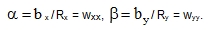
The Maxwell-Betti theorem α = β results in the equality (67) = (68), i.e.

(69)

which is identical with the equality (18) for physically orthotropic plates. However, in that case it was a result of a general symmetry of physical constants (8) that follows directly from the requirement that the potential energy of internal forces of the body be a homogenous quadratic function of stress components or deformation components.

Also in plates with shape orthotropy it must be ensured that the relation (69) is satisfied. If we use a technical reasoning or an experiment to determine e.g. coefficient μ₂₁ for the situation shown in Fig. 7a, also the other coefficient (for the situation in Fig. 7c) is determined.

(70)

Satisfying this relation does not result in large values of μ for technical materials that behave like physically orthotropic materials (plywood, fibreglass, etc.). For example one specific type of pressed plywood has

or another type of cross-glued plywood gives

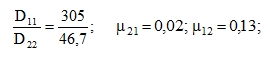
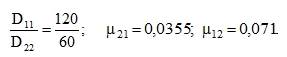
In practice, there may be a big ratio D₁₁/D₂₂ in shape-orthotropic plates, which may be in the range of 10 to 20.

Usually however, it is found that, at the same time, the coefficient μ₂₁ is very small, and therefore μ₁₂ does not exceed 0.5 or 1.0. With regard to the definition of μ₁₂,μ₂₁ by means of bending moments (Fig. 7), also values exceeding 0.5 or even 1.0 are not, in technical point of view, faulty. After all, they do not represent physical coefficients of contraction, which would be limited by volume changes of the substance. In real situations and with proper thinking about transverse moments, such values are really rare.

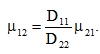
As the determination of the actual coefficient μ₁₂ or μ₂₁ can itself represent quite a difficult problem, simple approximate formulas are used in practice for what is called non-diagonal stiffness element D₁₂ that does not include these coefficients, but only the coefficient μ of the isotropic material that the plate is made of, for example  μ = 0.15 for concrete or 0.30 for steel. In ribbed plates and hollow core slabs, we can use the simplified formula (28):

(71)

or a similar formula (27) that, however, gives positive D₁₂ only for γ+μ>1 , which e.g. limits its application in concrete to situations when 0.85 < γ < 1that are however quite frequent.

Similarly, instead of (56) the simplified formula (23) can be used:

(72)

and the increased modulus of elasticity (41) is substituted into the formulas (53) to (55), which represents a broadly small increase of 2.25% in concrete and 9% in steel.

Conclusions from the previous paragraph 6.2.2.1 are applicable for the utilisation of values of M_xy.

Note concerning the plate mid-plane:

It can be seen in the previous figures that, generally, the centre of gravity of sections x=constant is located in a different distance e_x from the top fibre than the centre of gravity of sections y=constant e_y. Therefore, we may ask a question about where the mid-plane of the plate is located. This question disappears if we consider that we calculate with a two-dimensional plate continuum where e_x, e_y belong in fact among the “physical” properties. More serious error, however, occurs in plates with different ribs as a result of neglecting the planar stiffness of the top plate, or the area of thickness t. What proved useful for such situations is the Giencke formula for mixed stiffness (20)

(73)

that is based on the total torsional stiffness of the plate

(74)

And this can be used to determine the orthotropy constant (26); see [1], p. 38

Shear forces and reactions

Shear forces result from the requirement of moment equilibrium of a plate element around the y-axis and x-axis (Fig. 2):

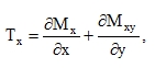
	(75)
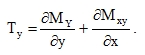
	(76)

After substitution of (16), (58), (59) we have

	(77)
	(78)

If we compare this formula with the fourth and fifth line of matrix (16) for physically orthotropic plates, we can see that instead of the mixed stiffness D₃ according to (20) the fourth line now contains the element

D3x = D12 + 2D33y

(79)

and the fifth line contains

D3y = D12 + 2D33x .

(80)

In the basic plate equation (25) - which is the condition of vertical equilibrium of a plate element

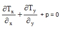
(81)

and simultaneously the Euler's differential equation of variational plate problem - the application of (79) and (80) changes the expression 2D₃ into the expression (D_3x + D_3y), so that we have the following formula for the determination of the value of D₃

(81)

 

Approximately (see 63a) we have

However, programs for physically orthotropic plates calculate T_x and T_y according to matrix (16). Values applicable for plates with shape orthotropy can be derived from these values only by means of a rather complex calculation. If we already know torsional moments M_yx and M_xy, this calculation can be inspected directly by (75) and (76). In both situations, the derivatives are substituted by differences of values in adjacent finite element nodes of the analysed plate and, therefore, we cannot get the full conformity.

The first members (75) and (76) prevail over the second ones in the larger part of the plan-area of common plates and, in addition, the difference between (79), (80) and (20) is not too big. Therefore, values T_x and T_y can be used for an approximate shear design.

The reactions of the plate are calculated from (29) or (30) also for the plates with shape orthotropy.

Plates with the effect of transverse shear taken into account

This is an analogy to short, high, etc. beams in which it is not possible to neglect the effect of shear forces T on the deformation, as that effect is comparable to the effect of moments M. This influences the shape of deflection line w(x) and thus also the values of all statically determined quantities, e.g. hogging moments that are decisive for the design.

Current programs have been developed for physically orthotropic plates following the paragraph 5.2 with the matrix of physical constants (33) and optional expansion into a full matrix of (5, 5) type in the case of a general anisotropy. Therefore, it is first necessary to transform a shape-orthotropic plate into a physically orthotropic plate, i.e. to determine constants D_ik in matrix (33).

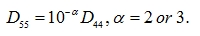
Instructions from paragraph 6.2.2 apply to constants D₁₁, D₁₂, D₂₂, D₃₃. What remains is to determine constants D₄₄ and D₅₅ in formulas

(82)

that specify the relation between shear forces and transverse shear components of deformation γ , i.e. the change of right angles between the normal of the mid-plane of the plate after its transformation into the flexural surface w(x, y), see Fig. 8. These deformations (32) are zero only if w_x = -φ_y, w_y = φ_x (see the sign convention, Fig. 1 and 8), i.e. the Kirchhof hypothesis (4) is valid.

The most important formulas are obtained if the transverse shear stress τ_xz, τ_yz is assumed distributed uniformly across the sectional area F_x, F_y of sections with the width of b = 1 constructed though planes x=constant and y = constant. For a ribbed plate in Fig. 8 we have

(83)

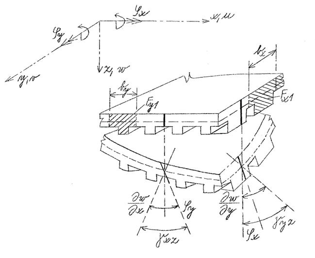
Fig.  8

In that case T_x = τ_xzF_x , T_y = τ_yzF_y , and with identical shear modulus G in both directions we have

D44 = GFx , D55 = GFy

(84)

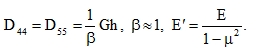
If there are no ribs in one or both directions and if the plate thickness is h, then in that direction

Fx = h , Fy = h ,  and thus in the solution of an isotropic thick plate	(85)
D44 = D55 = Gh.	(86)

These formulas are sufficient for the estimate of the magnitude of shear stress and for the estimate of required shear reinforcement in concrete.

More detailed analysis however requires that the actual distribution of shear stress τ_xz(z), τ_yz(z)  in interval -h₁  ≤ z ≤ h₂ be taken into account,  where h₁ + h₂ = h  is the plate thickness and h₁, h₂ the distance of extreme fibre from the centroid of the section. In plates with shape orthotropy, it is possible to use the well known Grashof – Zuravky formula (with plate indexes)

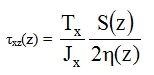
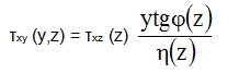
(87)

and similarly for τ_yz where 2η(z) is the width of a section in the point specified by the coordinate z, and S(z) is the first moment of the section above this width related to the horizontal centroidal axis (Fig. 9). In rectangular section of width η = 1 this formula gives the distribution τ_xz (z) that follows a parabola of the second order with its maximum in the centroid.

The same distribution can be obtained in isotropic plates in the Kirchhof theory (4) from Cauchy equations of equilibrium, and therefore, we can assume that the application of (87) in plates with shape orthotropy will be fairly accurate.

An uneven distribution of shear stress τ_xz (z), τ_yz (z) results in shear deformations γ_xz (z), γ_yz (z), distributed non-uniformly across the plate thickness.

If we introduce the assumption of a rigid normal (Fig. 8), the consequence is that we get constant γ_xz , γ_yz  and thus also τ_xz , τ_yz , and therefore the formulas (83) – (86) are justified. If we apply the more accurate distribution (87) and want to stick to the procedure of the finite element method, we have to find out the relation between T_x, T_y and values γ_xz , γ_yz, that are independent on z and represent angular changes in the sense of the equivalence of the potential energy of internal forces. For plates with shape orthotropy let us again proceed on the assumption of beam theorization: In a beam element of length l, in which a constant force T_x is acting, the accumulated potential energy is:

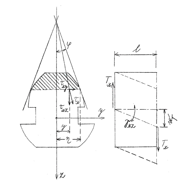
Fig.  9

If we substitute into this formula from the Grashof hypothesis τ_xz  (87) and

and from Hook’s law ,

we get

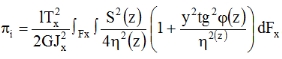
Let us introduce the usual formula for the energy with a corrective coefficient β that expresses the variation of τ across the section

	(88)
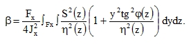
	(89)

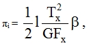
Let us write the energy (88) in the form of a half the product of the force T_x and path w_T (Fig. 9):

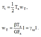
Then it is clear that a constant angular change, equivalent in terms of energy to variables γ_xz (z), is

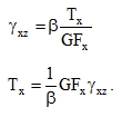
Instead of formulas (84) that are valid for a constant τ_xz across the whole section, we may use the following elements of the matrix of physical constants:

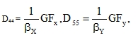
(90)

where subscripts β indicate that β can be different for sections x=constant and y=constant.

Box-sections

Thick-walled box-section – non-solid slabs

 

A non-solid plate with continuous hollow cores in one direction (let us denote it x) can be calculated as a shape-orthotropic plate with transverse contraction and thus formulas from paragraph 6.2.2 apply to it.

The assumption is that the webs of the box-sections are thick enough. Their thickness t_i (it can be even variable) should roughly satisfy the inequality

(91)

where h is the total plate thickness. If the vertical webs are thick enough (ratio b_s / b › 1/10 ), the influence of shear forces on the deformation of the plate can be neglected and the following formulas from paragraph 6.2.2 can be used to determine the matrix of physical constants (Fig. 10):

Section	β
Rectangle (plate without ribs)	6/5
Solid circle and approximately also solid n-angle (n ≥ 6)	32/27 (TP 3) 10/ 9  (ROARK)
Circle – thin-walled circular rings and approximately n-angles (n ≥ 6)	2
Steel I-beam no. 8 to 45	2.8 to 2.1
Concrete profiles: I, square, T, etc. with sectional area F and web area Fs, approximately	F/Fs
I-sections, squares, etc. with the sum of vertical webs thickness t1and radius of gyration to the neutral axis r:

The value J_x is calculated for section y=constant with a unit width that goes through the thinnest part of horizontal webs of the box-sections.

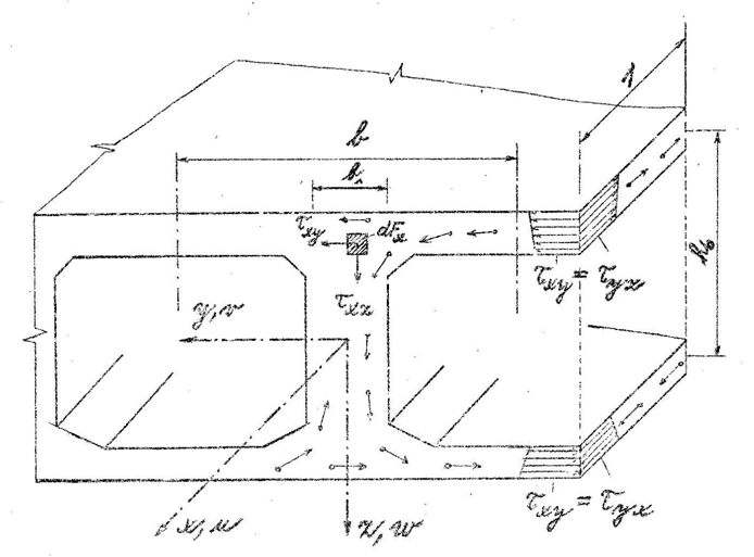
Fig.  10

Values Jxb are calculated for an I-section where the flange width b is always the distance between the vertical axes of the boxes. In case of unequal boxes also the I-sections are asymmetrical. Jxb is always related to the horizontal centroidal y-axis. The difference in the height of the centroids of sections x=constant and y=constant (see the note at the end of 6.2.2) is not significant. To determine the torsional element D33, also formula (63) can be used:

on condition that we take into account the remarks stated in paragraph 6.2.2 that are given after that formula. It means that the differences between (i) values J_kx, J_ky that follow from the Saint Venant torsion of beams and (ii) values J_kx ,J_ky relating to the actual shear flow by (58), (59) are in box-sections more significant than in plates with open ribs (Fig. 6b). In Fig. 10 the arrows and circles show the shear flows that approximately occur due to the necessity to keep τ_xy =τ_yx. In closed box-sections with vertical webs thick enough, shear circulation may develop and the corresponding J_xk from the beam-based calculation will be broadly accurate. The circulation in the top and bottom part of the section y=constant will be however analogous to Fig. 6b, it will be strongly suppressed and the torsional moment will be approximately defined by the pair of horizontal forces V_x with the lever arm h₀. What is important is whether there are transverse diaphragms in the plate and what the distance between them is, as the shear flow is affected in their vicinity. If the diaphragms are distributed close to each other, box-sections are again in fact formed in sections y=constant and their J_ky, relating to a unit width, will be decisive for the calculation.

Thin-walled box-sections

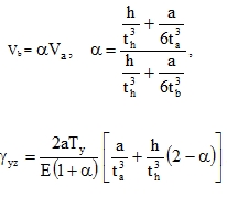
They can be approximately analysed as plates with the influence of transverse shear taken account. In this analysis we use input data based on the comparison with modified formulas of V. Křístek:

(92)

where J_xa is the moment of inertia of the I-section of width a (Fig. 11) between box axes. It may however vary across elements, i.e. different boxes. The stiffness D₂₂ is not too overestimated as the influence of the web J_xa is small. Similarly, D₃₃ is quite accurate especially in internal boxes, as the amount of shear flow that gets into the internal thin webs is very small. We may approximately calculate with a proximate value where t is the thickness of horizontal plates and h is their centre-to-centre distance. For unequal thicknesses this value may be approximately determined from formula (96) presented later.

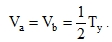
The shear stiffness D₅₅ in transverse direction y (see the fifth line of the matrix (33)) can be found through the comparison of the formula T_y = D₅₅γ_yz with the formula defining a relation between the transverse force

Ty = Va + Vb

in the highlighted I-shape frame of unit width and total skewing γ_yz = γ₁ + γ₂ where γ₁, γ₂ are beam deflections of webs and flanges. Taking dimension as in Fig. 11 we get

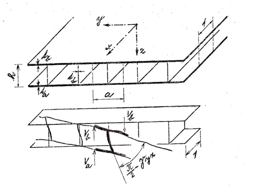
Fig. 11

(93)

Therefore:

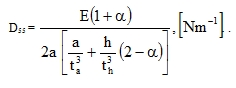
(94)

The shear modulus G₂₃ (paragraph 5) was not needed for this calculation, but it could be determined for the substitute physical plate continuum e.g. on the assumption of (34) from the formula G₂₃ = D₅₅ / h without introducing the conception of a sandwich plate with a soft core.

Stiffness D55 is substantially increased in the location of transverse diaphragms. If they are very rigid and if they provide for non-deformability of the section projection into the vertical plane, then γ_yz can be neglected in elements located in the vicinity of these diaphragms (see the procedure for D₄₄). This should happen with reasonably designed diaphragms, the web stiffness of which is higher by a factor of ten in comparison with the previously stated stiffness. The variation of D₅₅ over elements can be easily taken into account in FEM. In case of densely located diaphragms, if one diaphragm relates to each finite strip, we can calculate with the average value of D₅₅, but the effect of shear γ_yz will be small, otherwise the diaphragm would not meet one of its main purposes.

The stiffness D₄₄ (4^th line of the matrix (33)) is according to (95) larger than D₅₅ by a factor of ten and the shear changes γ_xz can be neglected. In the input it can be expressed by the value

It could be also possible to modify the program for plates with the effect of shear in one direction that nullifies γ_xz beforehand.

Processing of printed internal forces:

Mx [N] ....	per one I-section according to Fig. 11 we have M = a Mx , stress       σx= Mz / J , extremes    σx = ± M / W .
Tx [Nm-1] ....	similarly, per one I-section, we have T = aTx , stress τxz  according to (87),  approximately for very thin webs τxz = T / h th  only in the web.
My [N] ....	In the top and bottom plate, axial forces in the transverse y-direction will become apparent Ny = ± My / h and stress σyb = -My / h tb,  σya = My / h ta.
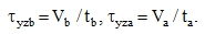
Ty [Nm-1] ....	In the top and bottom plate, the transverse shear forces Vb and Va will occur following from (94), i.e.  Va = Ty / (1+α), Vb = αVa , with identical plate thickness. The transverse shear stress is approximately:
Mxy [N] ....	In the top and bottom plate, the horizontal shear forces Txy = ±Mxy / h occur and stress τxyb = Txy / tb ,  τxya = Txy / ta .

These values can be used in steel plates to calculate principal stresses that can be used for the assessment of their safety. It is similar in reinforced concrete structures (thin-walled), where the tension is carried by normal or prestressing reinforcement and the effect of M_xy is reflected in the design moments, i.e. in the substitution of M_x , M_y  by  M_xdim, M_ydim .

Comparative example

In order to compare the input data D_ik, let us discuss an example of a deck slab box-section of the overbridge C 201 in Vsetín, Czech Republic, made as a prefabricated lamellar structure.

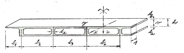
Fig.  12

The division into finite elements was selected to coincide with the plan-view of the boxes, which means that the stiffness of elements was based on the stiffness of individual boxes. The transverse section is schematically shown in Fig. 12 that would be more complex due to the varying thickness of webs. The calculation according to paragraph 6.4.1 – thick-walled structures – (92): Moments of inertia of individual boxes J_xb were found by means of a program for the calculation of geometric characteristics of planar shapes. Moments J_y can be easily calculated using the formula

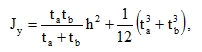
(95)

where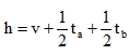 is the centre-to-centre distance of horizontal webs.

Vertical webs are of unified thickness 30 cm and their centre-to-centre distance is 300 cm. Further, let us give the approximate dimensions of the box b₃ in [cm]: t_b = 18, v = 96, t_a = 14, h = 112 and the same for box b₄: t_b = 19.5, v = 101.5, t_a = 14, h = 118.

Physical constants E = 385000 daN/cm² (kp/cm²), μ=0,15.

The stiffness matrix of box b₄ (higher numbers by (92) – thick-walled, lower numbers by (93) – thin-walled neglecting the vertical webs):

	509 809	70 316
	448 000	67 100	0
	70 316	431 038		10 kNm
D=	67 100	448 000		(Mpm)
			199 228
	0	0	224 000

 

For box b₃ :

	475 046	64 720
	389 000	58 300	0
	64 720	391 887
D=	58 300	389 000	0
			183 374
	0	0	194 500

The reduction of the flexural stiffness D₁₁ by neglecting the vertical web is apparent; the stiffnesses D₂₂, D₃₃ will be larger, which follows from the thin-walled theory. The differences in moments (multiples of type D₁₁w_xx etc.) will be smaller, as the larger D₁₁ gives smaller deflection w and also smaller derivative w_xx. It is known that moments in isotropic plates do not depend on D at all if we consider only the action of forces. This independence is of different nature in orthotropic plates: the moments do not depend on the absolute values of D_ik, but on their ratios. The most typical ratio for this relation is

see (26). Examples of the influence ofχon moments can be found in [ 1 ], pp. 48., table 2 and in diagrams in Fig. 13, p. 52.

Multi-cell slabs with linear hinges in longitudinal direction

This means perpendicular or oblique plates assembled from prefabricated blocks, in which we assume that no reliable monolithic connection exists in the transverse direction (e.g. through transverse prestressing, which would cause that they would be treated as monolithic plates in accordance with the previous paragraphs).

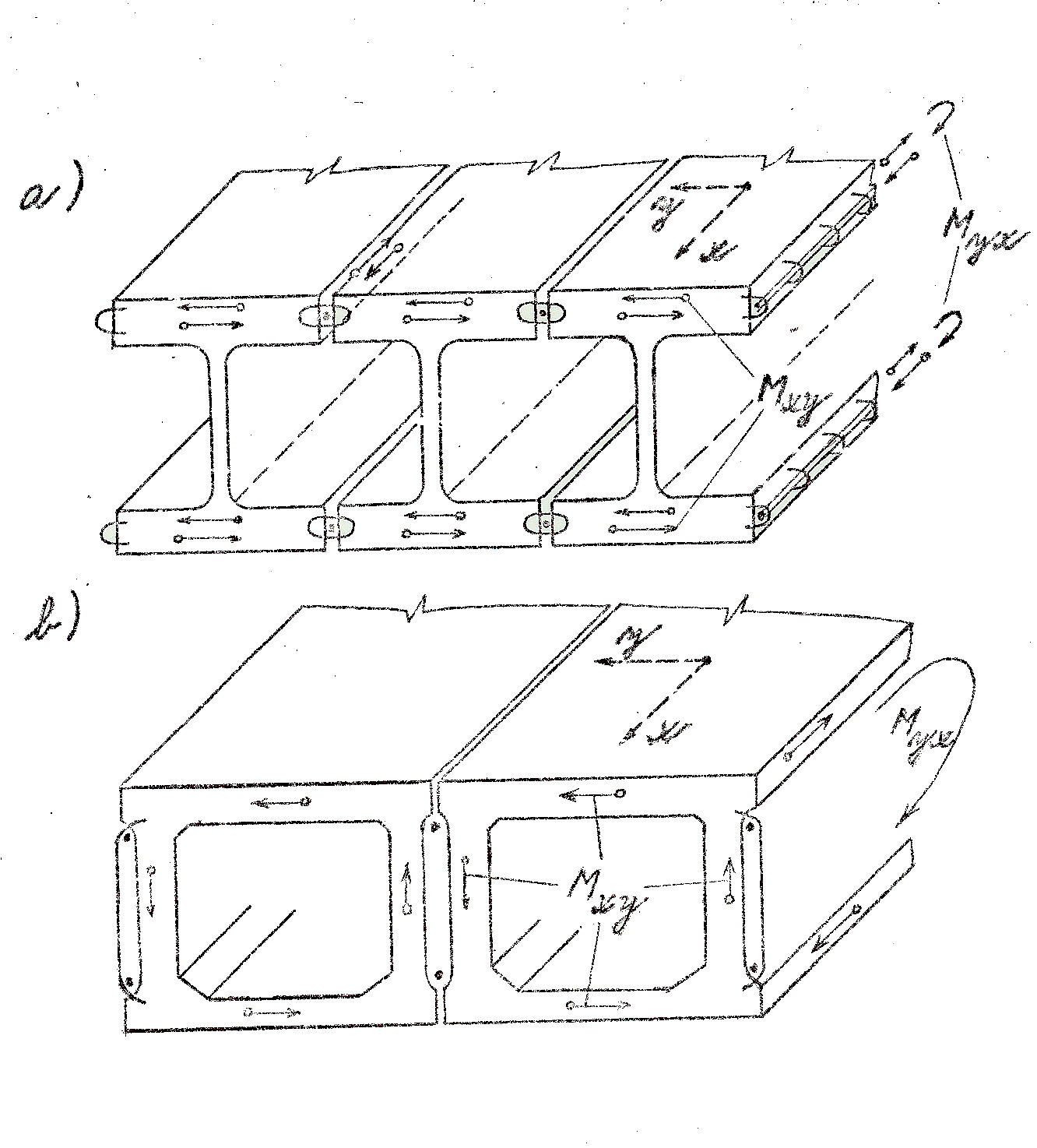
Fig.  13

Longitudinal joints transfer only shear forces T_y and no bending moments M_y.

There are many types of multi-cell slabs with linear hinges in longitudinal direction. In terms of input data D_ik, all of them fall between two limit situations (Fig. 12):

a) The vertical webs of the box-sections are so thin that practically no shear flows gets into them and the torsional moment M_xy transfers only the shear in the top and bottom web. Then we may consider the equality , and therefore, following from (63), the torsional stiffness is

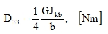
(96)

if we calculate J_kb [m⁴] for one prefabricated block of width b [m].

Similarly to box-sections, the formula (92) applies to other stiffnesses.

b) The vertical webs of the sections are so thick that a continuous circulation of shear flow occurs in sections x=constant, which (considering the theorem of reciprocity τ_xy = τ_yx ) influences also the shear flow in sections y = constant. Then, we apply the formula (63) with varying torsional stiffnesses J_kx , J_ky [m³] and constant shear modulus G:

c) A special situation arises when the longitudinal joints cannot transfer any torsional moment. Then we have J_ky = 0 ,

Formulas (62) generally apply to the evaluation of printed M_xy.

If the webs in plates in Fig. 13a are so slim that transverse skewing occurs, the appropriate stiffness D₅₅ from paragraph 6.3 can be found on the basis of the formula (95) from paragraph 6.42.

Other plate types

Reinforced concrete plates with different reinforcement F_ax, F_ay in x- and y- direction behave in the first phase practically like isotropic plates until cracks form in the tensile part of the concrete. In the second phase, we have to find moments of inertia J_x, J_y of the non-homogenous sections of unit width composed of (i) steel and (ii) concrete in compression. The ratio J_x/ J_y is approximately equal (plus or minus a few per cent) to the ratio F_ax/ F_ay. As the zone of concrete in compression, where some transverse contraction (or dilatation) still occurs, is small, the effective value μ is lower than 0.15. The value 0.02 was measured. The stiffnesses are calculated from the formulas stated earlier

	(97)
	(98)

The effect of shear is taken into account only in plates whose thickness h › L / 5, see paragraph 5.2 and 6.3. Deviations that are of practical significance occur only if h › L/3.

Corrugated plates are calculated using the formula (98), and for sinusoidal shape of sections x = constant we take:

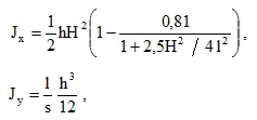
(99)

where the shape of the corrugation is z = H sin πx / l, the thickness of the corrugated plate is h, the amplitude of waves is H, and the length of the chord of one half-wave is l. This can be used approximately also for non-sinusoidal shape of the waves. Doubled corrugated plates (system BEHLEN, PUMS, etc.) require a special calculation of J_x. In extra-thin corrugated plates, J_x can be calculated on the curve z = f(x) and then multiplied by the thickness h. The ratio J_y / J_x is almost zero.

Double-layer braced plates are beam systems used for roofing of extensive areas (stadium, etc.). For the needs of a preliminary calculation, they can be considered as orthotropic plates, with moments of inertia derived from sectional areas F_ax , F_ay  of the beams in strips in x- and y- direction and lever arms r_x , r_y  to the centroids of these areas, approximately It is possible to establish the effect of  transverse shear similarly to paragraph  6.3. The torsional stiffness is practically zero (D₃₃ = 0, χ = 0 ) in common right-angled systems of strips without diagonals in horizontal planes; in other systems it must be determined by means of comparative calculations. The printed values M_x, M_y, T_x, T_y can be used for the calculation of axial forces in beams by means of the procedure that is common for lattice girders (intersection method). The procedure can be extended to generally anisotropic plates and is suitable for a preliminary design or for the determination of an optimal variant, etc. After the final design of the system, the accurate assessment can be performed following the calculation of axial forces in beams of the given system. The beams are, depending on the nature of joints, considered as a three-dimensional lattice girder or as a frame.