Surface Loads (2D results)
The Surface Loads command serves for displaying surface loads applied on 2D members in project.
Usage
- Calculate a FEM analysis of the model
- Go to Results > Surface Loads
- Set properties of the command to specify mainly:
- Click on [Refresh] action button to display the results
Properties
| Category | Property | Description / Notes |
|---|---|---|
| Selection |
Type of selection
|
Specifies on what members the results are displayed
|
| Filter
No / Material / WildCard / Layer / Thickness |
||
| Result case |
Type of load
|
Defines for what load the results are displayed. See "Result case" |
| Extreme | Location
In centres |
Not possible to be changed, not depicted in the properties. Entity value (2D surface load) is the same through the whole element. Also see the chapter "Mesh dependency" below |
| Extreme
Member / Global |
Defines for which extreme on 2D member the results are displayed. | |
|
Values |
q_x, q_y, q_z | |
| System | System
LCS mesh element / Global |
Sets a coordination system which is used as referenced for displaying the results. |
| Errors, warnings and notes settings | "Errors, warnings and notes settings" | |
| Drawing Setup 2D | "Drawing setup 2D" |
Legend
Two types of legend are automatically available in 3D scene.
If in selection there are only 2D mesh elements with less than 20 different values of surface loads - legend with separate values is displayed.
If in selection there is at least one 2D mesh elements with more than 20 different values of surface loads - continuous legend with range is displayed.

Behaviour and features
Mesh dependency
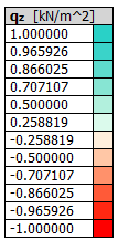
The graphical depiction of the surface loads depends on mesh size. Only surface load of those mesh elements is depicted, where the load (for example generated free load) covers more then 50% of that element surface. An example is provided in the figure below.
Note: this does not mean the load is not being applied in these elements. It is applied internally as nodal forces, but these are not depicted graphically.
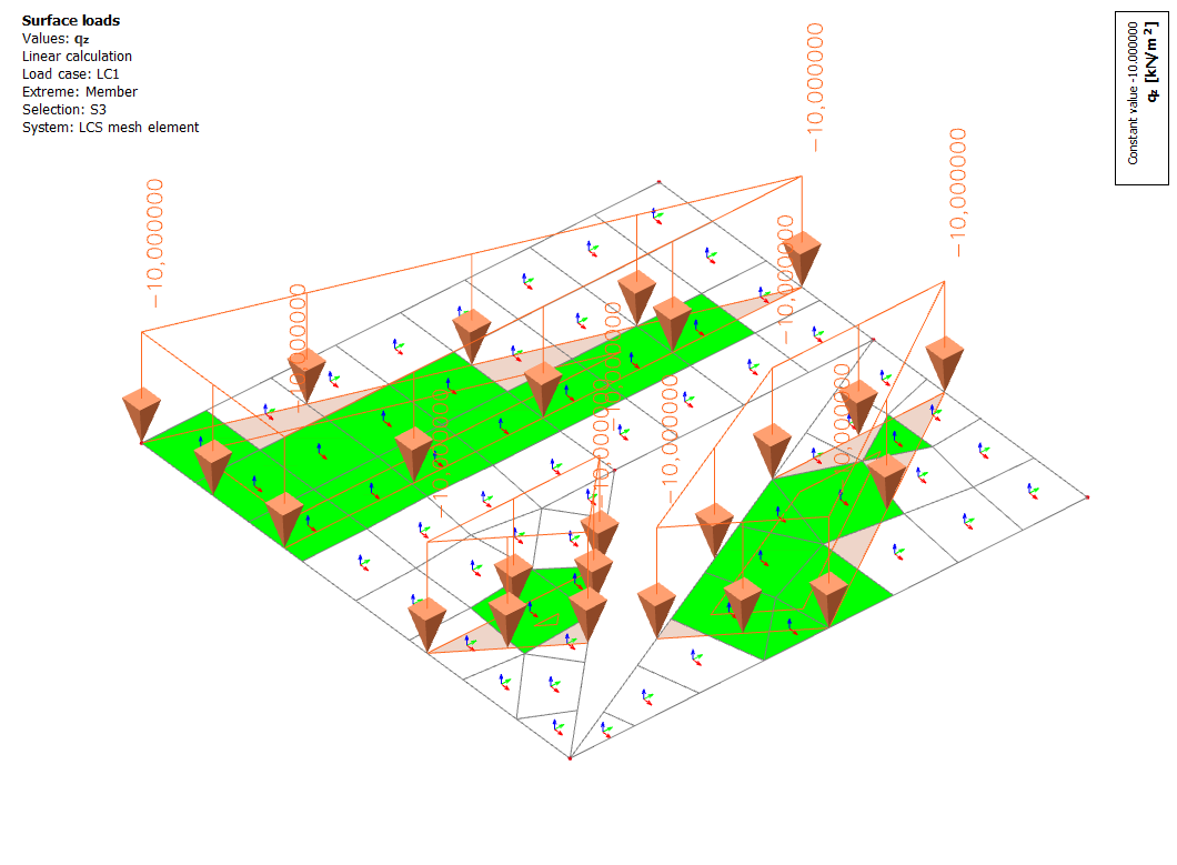
For finer mesh:
The condition of at least 50% loaded area is evaluated for each (generated free) load separately. Even if the two (or several more) free loads have the same value.
For example, there are 2 cantilevers, #A and #B. Mesh size is 500 mm. One free load is applied on a structure #B. However, more (in this example 4), the same value free loads are applied on a structure #A.
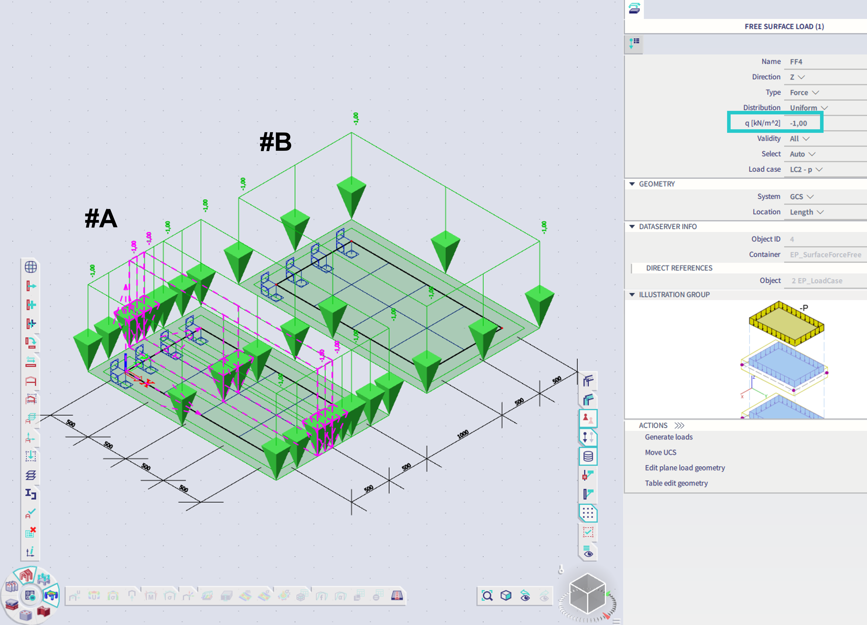
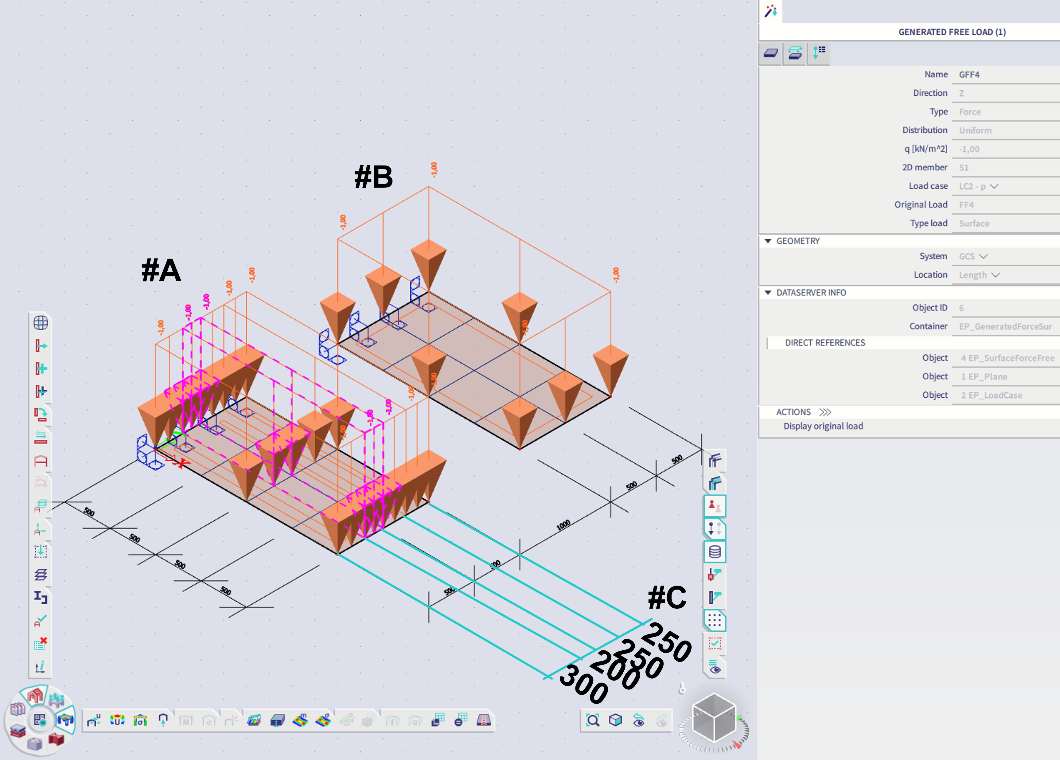
The generated loads from these free loads are depicted in the figure below. On structure #A, there are 4 strips of 300, 200, 250 and 250 mm (#C).
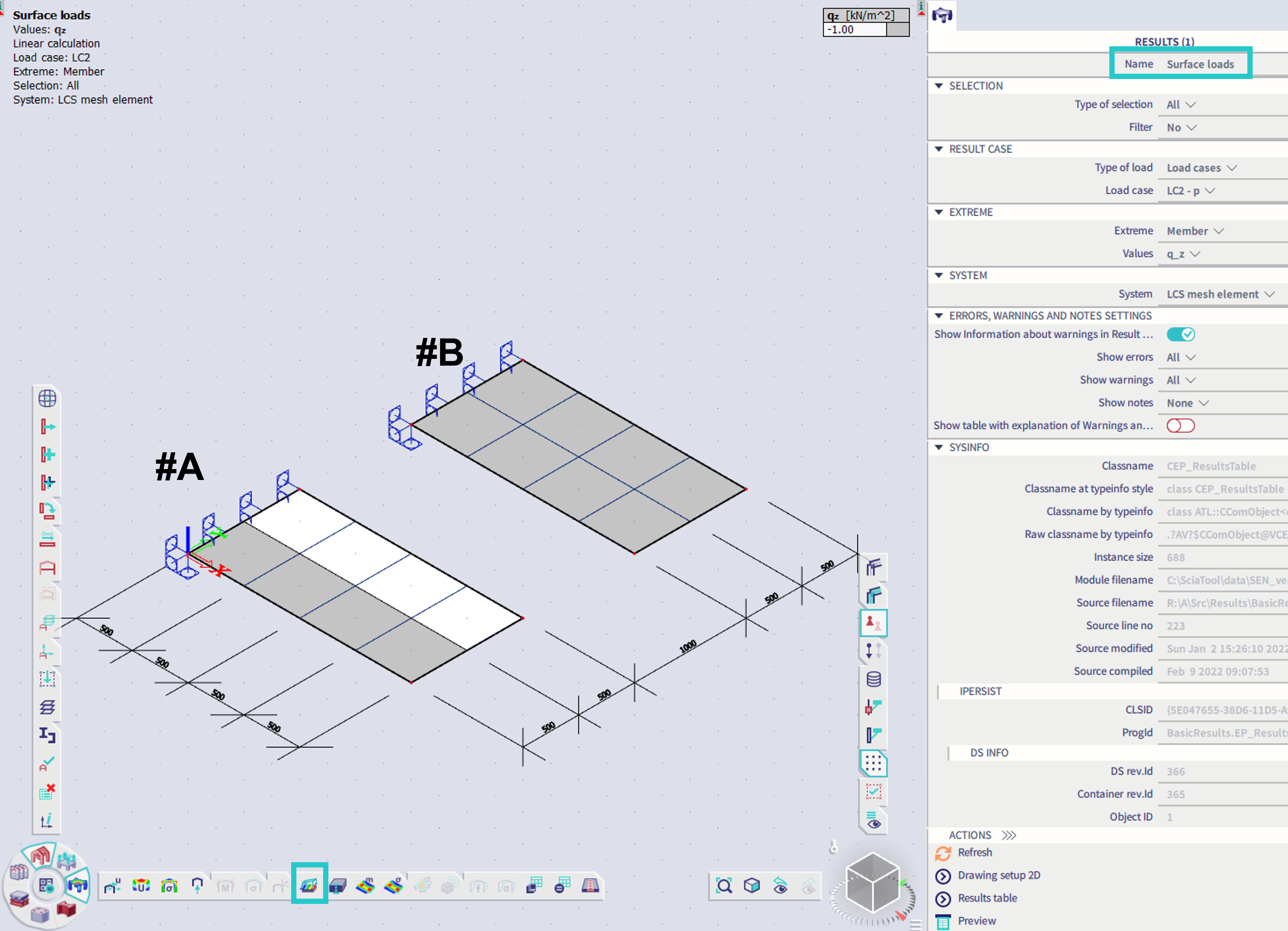
If the "surface load" is to be checked after the calculation, the result is as follow:
All the elements are depicted as loaded by the surface load in case this surface load origins from one source ( #B).
In case #A, the finite elements are practically loaded by the same value (1 kN/m^2). Only those, which were loaded by a load generated on more then 50% of surface area, and that load origins from one load-source are graphically depicted. Therefore in the example below, those with 300 mm width out of 500 mm.
Note: this is due to fact, each load source is evaluated separately for loading of mesh element (as the load sources might have a different value). The condition to check for equal neighbouring values of load sources would slow down the process in general, and would be rather contra productive. This case is considered rather as special one, not so frequent, therefore in order not to slow down the whole process, such condition is not implemented.
The load which is not considered as "surface load" on mesh elements (load at the white part of the #A in figure above) is applied as a nodal force (nodal forces are not yet possible to be graphically depicted).
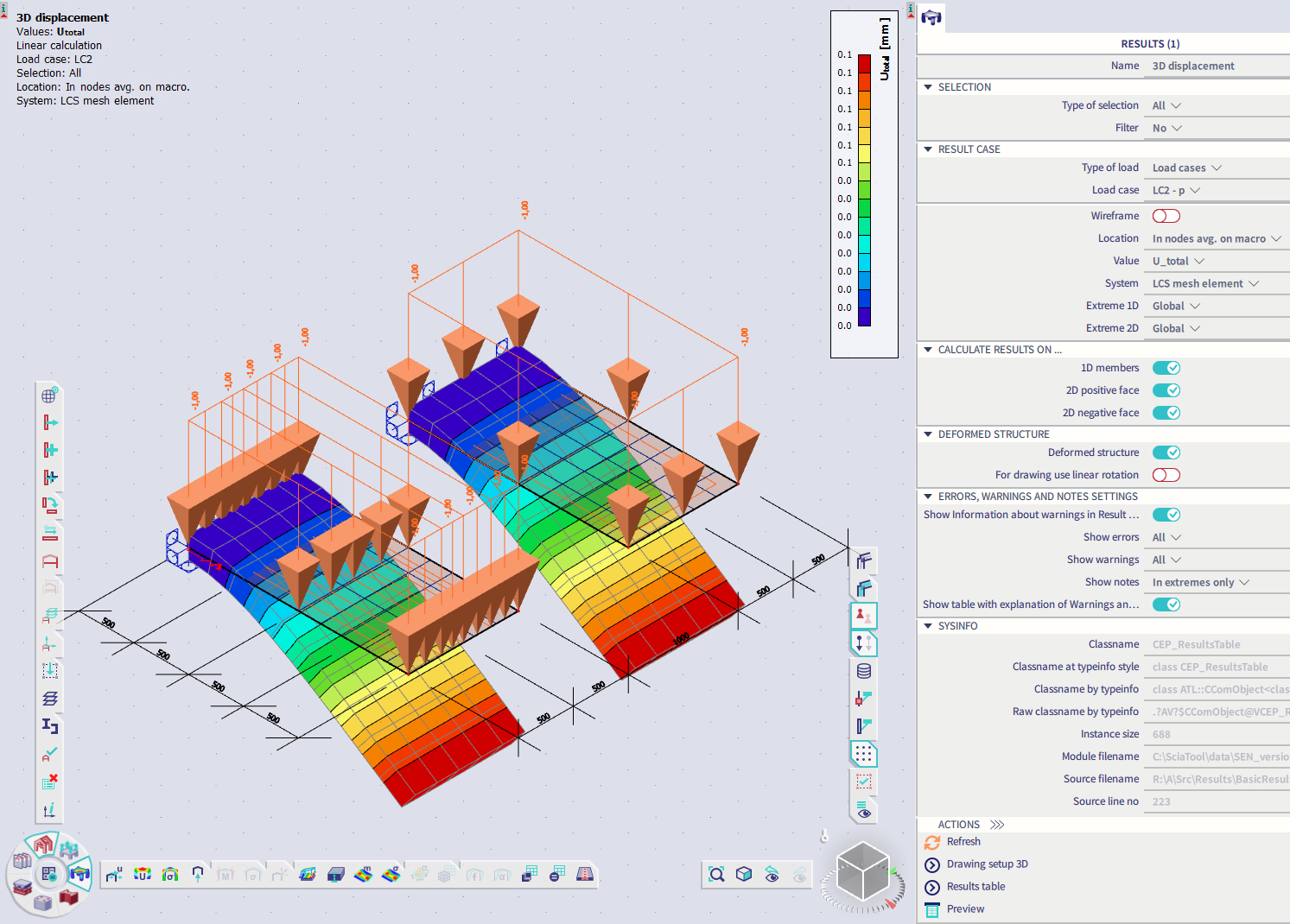
The displacements are of course the same for both cases:
Nonlinear combinations
It is possible to plot the surface loads for nonlinear combination where the initial imperfections are applied, what might be helpful if there are also free loads in the model.
For example let's assume a structure like below, a slab supported by 2 walls at each end, and a load case (LC4 in example) to implement an initial imperfection.
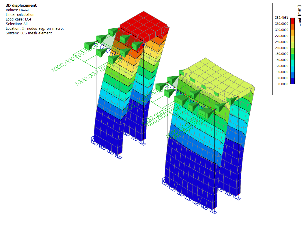
A nonlinear combination is defined (NC1), with the global imperfection based on the deformation from LC4
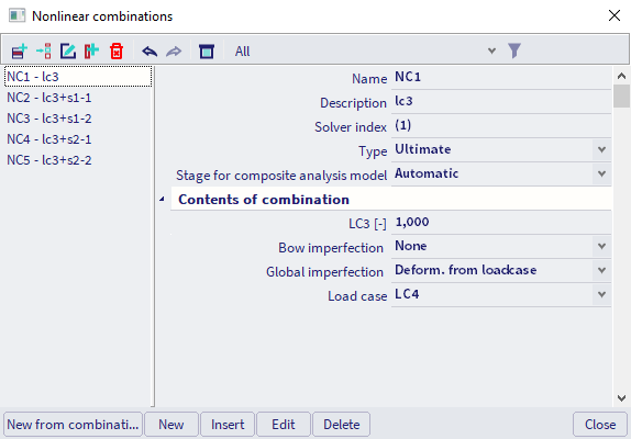
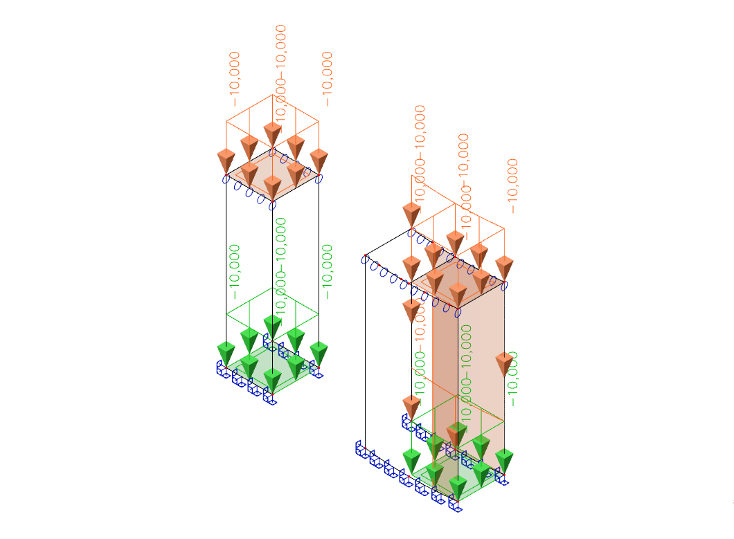
The nonlinear combination (NC1) contains a load case LC3, which contains a free surface load modelled as:
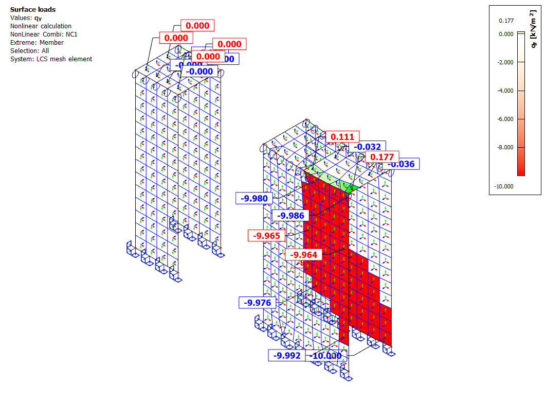
Notice that the right structure has slightly rounded walls (circular arc with large diameter)
When the NL analysis is initiated, this warning appears:

With the 2D surface loads, it is possible to check what elements have been loaded, as the free loads in combination with global initial imperfections is applied on deformed structure in case there are structural elements (slabs, walls) to be applied on. However, in case load panels would be used, the free load is generated on the initial geometry of these load panels (even if the initial imperfection of surrounding structural members is implemented)
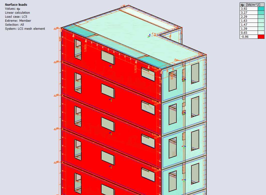
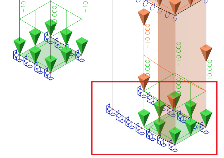
For example in this case q_y surface load in LCS of the mesh elements is:
Or q_z surface load in LCS of the mesh elements is applied as:

In order to see the applied surface loads more precisely, a finer mesh is required (see chapter above).