Sample input of a load pattern on a track
The below is an example of a proper input procedure for the definition of a train load (or, generally speaking, load pattern moving along a track).
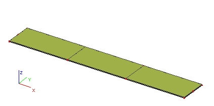
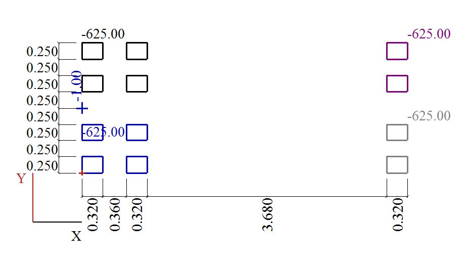
First, we input a simple structure composed of three slabs in a row (from left to right: S1, S2, and S3).
Second, we define a track in the middle of this strip (function Load >Traffic loads > Traffic lane).
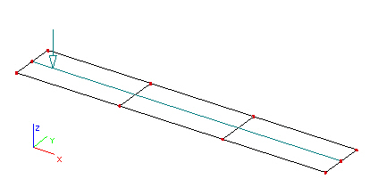
When the track is input, we can adjust its parameters in the Property window.
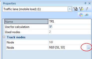
What deserves a special attention is the node list under Track nodes section of the dialogue. The list contains all the nodes of the track in question. Especially the last node of each interval of the track is very important. In our example we have input a single-interval track. In practice, the track may be defined as a polygon. In that case, each end-node of each interval is of the same importance.
The three-dot button at each end-node opens a dialogue that defines the "validity" of the particular track interval. It means that we can select only certain slabs from the model that will be subjected to the generated train load. Slabs not included into this list will not be affected by the load generated on the track interval.
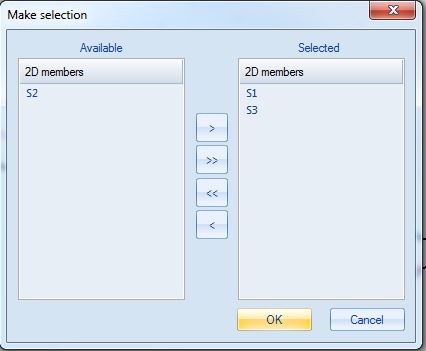
In our example, we define that the load track is "valid" only for slabs S1 and S3 (Slab S2 thus will not be subjected to any generated mobile load).
Next, we define the load pattern that will move along the track (function Load >Traffic loads > Single Traffic Loads).
In our example we create the following load pattern.
Finally, we can let the program to move the load pattern along the track and generate a new load case for each position of the load (function Load >Traffic loads > Lane loads manager).
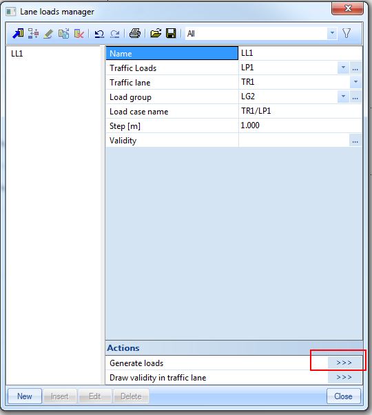
The program generates a set of new load cases. Each new load case corresponds to one position of the mobile load. In our example we get 36 new load cases (the structure is 33 m long. the load pattern is 5 m long and the step for the "move" of the load is set to 1 m).
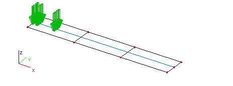
Load position 1 = load case LC1:
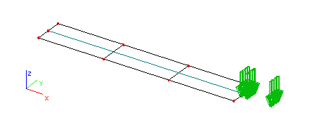
Load position 36 = load case LC36:
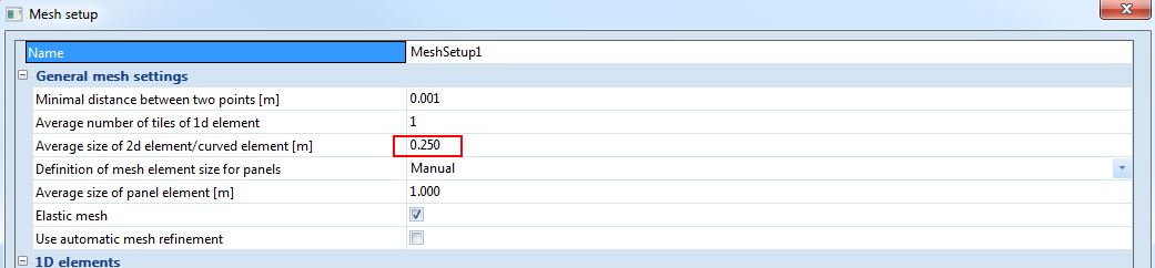
As the next step, we have to generate the finite element mesh so that the program can accurately distribute the load in the generated load cases to the slab. It is important to set the right size of the finite elements (function Calculation, Mesh > Mesh setup).
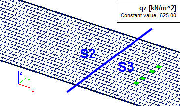
When the finite element mesh is generated, we can check the input data and see how the program distributed the load patterns (formed by point loads) to individual finite elements (area load). We can also check that this distribution of load takes account of the "validity" of individual track intervals. In our example we will see that the middle slab S2 will not be subjected to any generated load.
In order to perform the check of the input data, option Test of input data in function Calculation, Mesh > Calculation must be started.
Once this check has been completed, a new function appears under Calculation, Mesh > 2D data viewer.
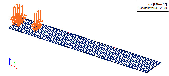
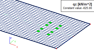
The generated and distributed load for LC1 (the green elements are those that are subjected to the calculated area load):
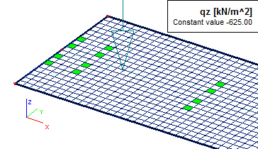
The generated and distributed load for e.g. LC33:
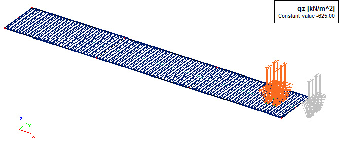
And finally, we can check that slab S2 is not subjected to any load generated during the above-described procedure. Let us take e.g. load case LC22.
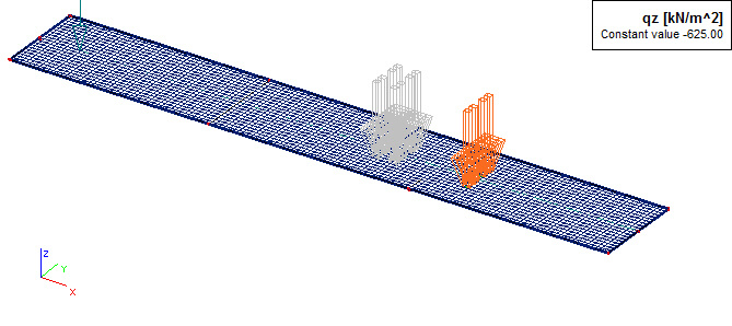
The load located over slab S2 is displayed in grey colour and it generates no area load in the finite elements of slab S2.
It is important to take in mind two important rules: (1) The procedure described above must be strictly followed. First, the validity of the track intervals must be adjusted and only then the load pattern can travel along the track. (2) The size of the finite element mesh must be properly set. Otherwise, nothing is displayed in function 2D data viewer.