FEM - Multi Freedom Constraints (MFC) - Lagrange Multipliers

Introduction

This chapter is to provide a closer information about newly introduced global analysis setting (found within "advanced solver settings") named "Use Lagrange Multipliers". This setting was introduced for SCIA Engineer version 24.0.

Option "Use Lagrange Multipliers" is turned off by the user

This option is the default setting. If the "Use Lagrange Multipliers" is off, so called "Penalty method" is used to treat the Multi Freedom Constraints (MFC), e.g. for rigid links, nodal constraints, etc.

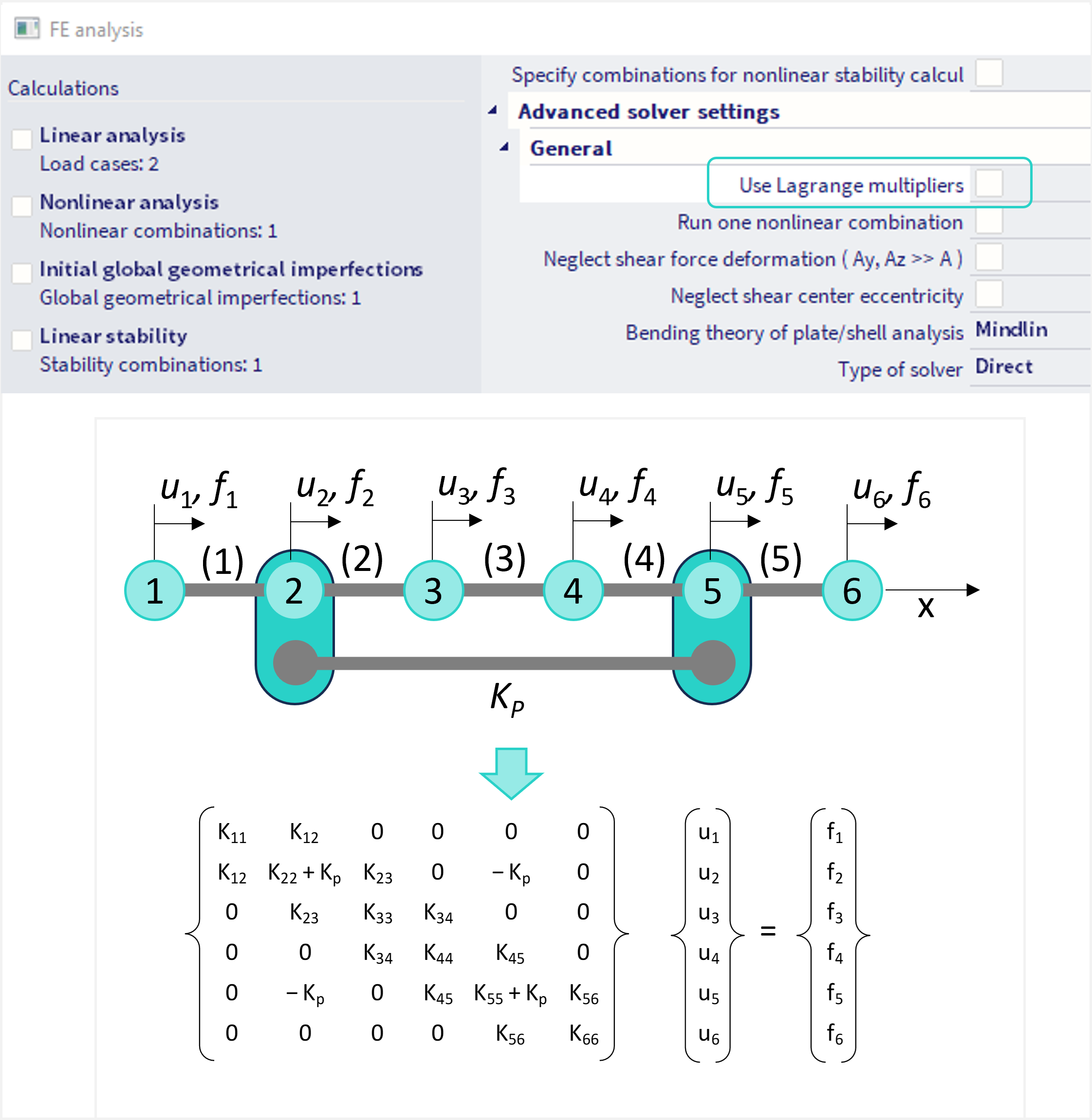
An example is provided below, on a structure of 6 nodes connected by 5 beams, where the only degree of freedom is along the x-axis. Node 2 and 5 are connected by a rigid link (aiming to get displacements u₂ = u₅). In this case, this constraint is internally treated by "penalty element" of stiffness K_P, which is much larger (by several orders of magnitude) then the stiffness of the other members. Stiffness matrix is provided in the figure below. Upon numerical solution however, the condition of u₂ = u₅ is satisfied approximately in the sense, there is non zero difference, so called "gap error" e_g = u₂− u₅. The larger the stiffness K_P, the smaller the gap error e_g. However, as K_P approaches ∞, columns 2 and 5 (as well as rows 2 and 5) become linearly dependent, hence the matrix approaches singularity (increasing the solution error). There are two effects at odds with each other. The most suitable K_Pis one, where these two errors (solution error and gap error) are roughly equal in absolute value. So called "square root rule" is utilized.

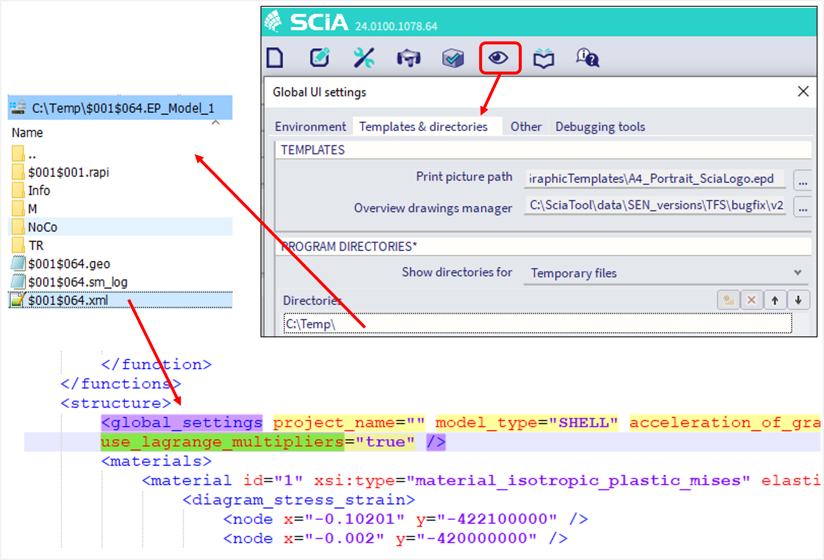
Note: in some cases, the usage of Lagrange multipliers is turned on in the background even if explicitly turned off by the user. This is done in case there are rigid diaphragms present in the project, as this option is recommended in general. The user might check the real consideration of this setting in the XML file which is sent to the FEM solver. This XML is to be found in the TEMP folder, and the path to TEMP folder might be seen in the global UI settings - see the example in the figure below.

Option "Use Lagrange Multipliers" is turned on by the user

In case the option "use Lagrange Multipliers" is on in the "Advanced solver settings", the "Lagrange Multiplier Adjunction" is used to treat the Multi Freedom Constraints (MFC), anywhere it is applicable (for rigid links, nodal constraints, rigid nodal supports, etc.).

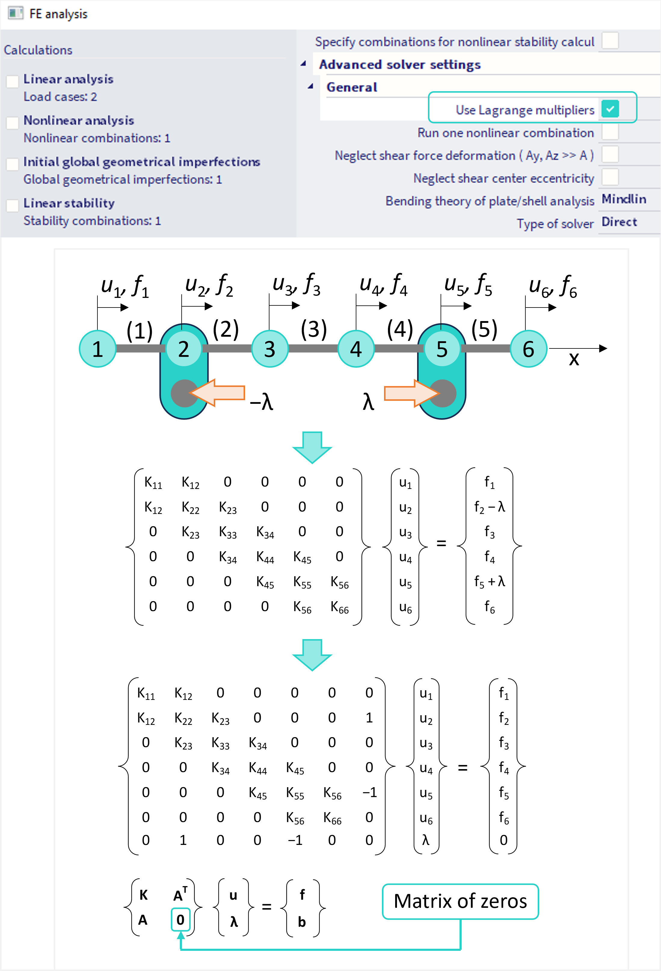
An example of the same case is provided below. Constrain of u₂ = u₅ is imposed exactly, as the nodes 2 and 5 are connected by an ideally rigid link rather than by one with very large stiffness. This ideally rigid link is replaced by an appropriate reaction force pair (−λ,+λ), so called the "constraint forces". λ is called a Lagrange multiplier. Because λ is an unknown, it is transferred in to the left hand side of the system of equations by appending it to the vector of unknowns, and the constrain u₂ − u₅= 0 is added as the seventh equation. This is multiplier-augmented system. The symmetric coefficient matrix is "bordered stiffness matrix". However, there is a zero sub-matrix in the right bottom part of this system, where 0 numbers are also on diagonal. The advantage is, that by solving this system, the desired solution for the degrees of freedom is provided, while the constraint forces are also characterized through λ.

Recommendations

Both options have some pros and cons. In general, use of Lagrange Multipliers might significantly improve the convergence of the nonlinear analyses and make the calculations more stable. However, due to the 0 elements on diagonal in the stiffness matrix, it is not recommended to be used for the modal analysis with Lanczos solver. In case use of Lagrange Multipliers is on, Polynomial solver is much more suitable in order to conduct modal analyses. Alternatively, for purpose of modal analysis, the use of Lagrange multipliers might be turned off, hence the penalty method will be used.