Nonlinear stability analysis (improvements since SCIA Engineer version 24.0)
Introduction
This chapter provides detailed information about nonlinear stability analysis, as it was reworked and significantly improved since SCIA Engineer version 24.0. In case older project with nonlinear stability combinations is opened in newer version, this warning will be shown:

Requirements
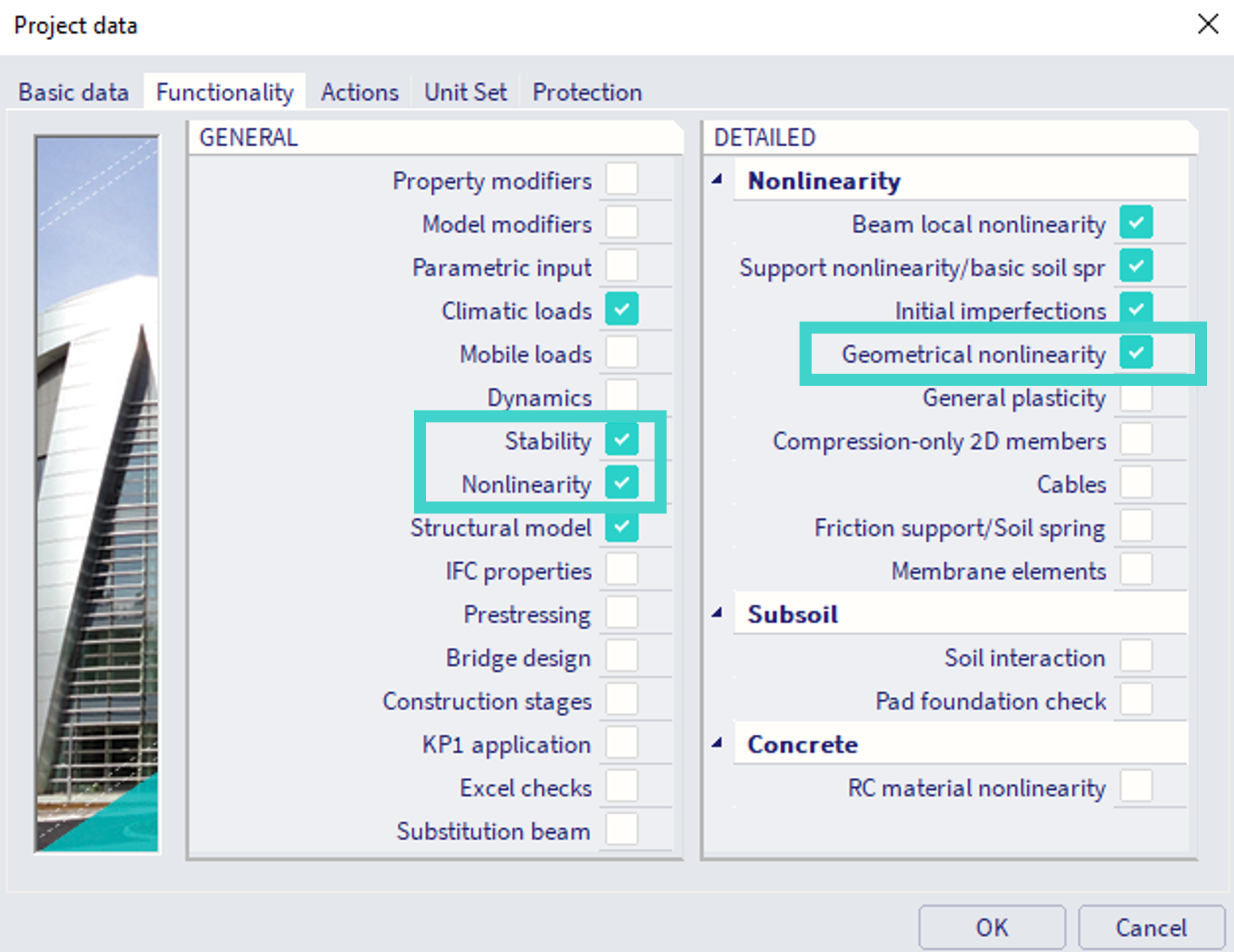
Functionality "stability"and "nonlinearity" must be on in order to define the nonlinear stability combinations (NL.ST.C.). Furthermore, in order to calculate these nonlinear stability combinations, the "geometrical nonlinearity" must be all activated as well. There will be a warning notifying user if nonlinear stability analysis is to be initiated without geometrical nonlinearity.
Basics of nonlinear stability analysis
During the nonlinear stability analysis, the content of the analyses combination is being added in increments. This is the same logic as in case of nonlinear analysis. However, the difference is, that the content of the nonlinear stability combination might be increased over 100% of the combination content, and when the process of the incrementation is ended (due to conditions explained further), the subsequent eigenvalue buckling analysis (linear stability analysis) is conducted using the deformed geometry and the stress state from the last increment of the previous corresponding nonlinear analysis (within nonlinear stability analysis).
It might be concluded that:
Nonlinear analysis (calculation of nonlinear combination) = nonlinear analysis up to 100% of the content of the corresponding combination
Linear stability analysis (calculation of linear stability combination) = linear analysis of the linear initial state (in the background) + subsequent eigenvalue buckling analysis
Nonlinear stability analysis (calculation of NL.ST.C.) = nonlinear analysis which might go over 100% of the combination content (in the background) + subsequent eigenvalue buckling analysis
Nonlinear stability settings
The settings of nonlinear stability within the solver settings are certain combination of settings for nonlinear analysis and linear stability, and are depicted in the figure below:
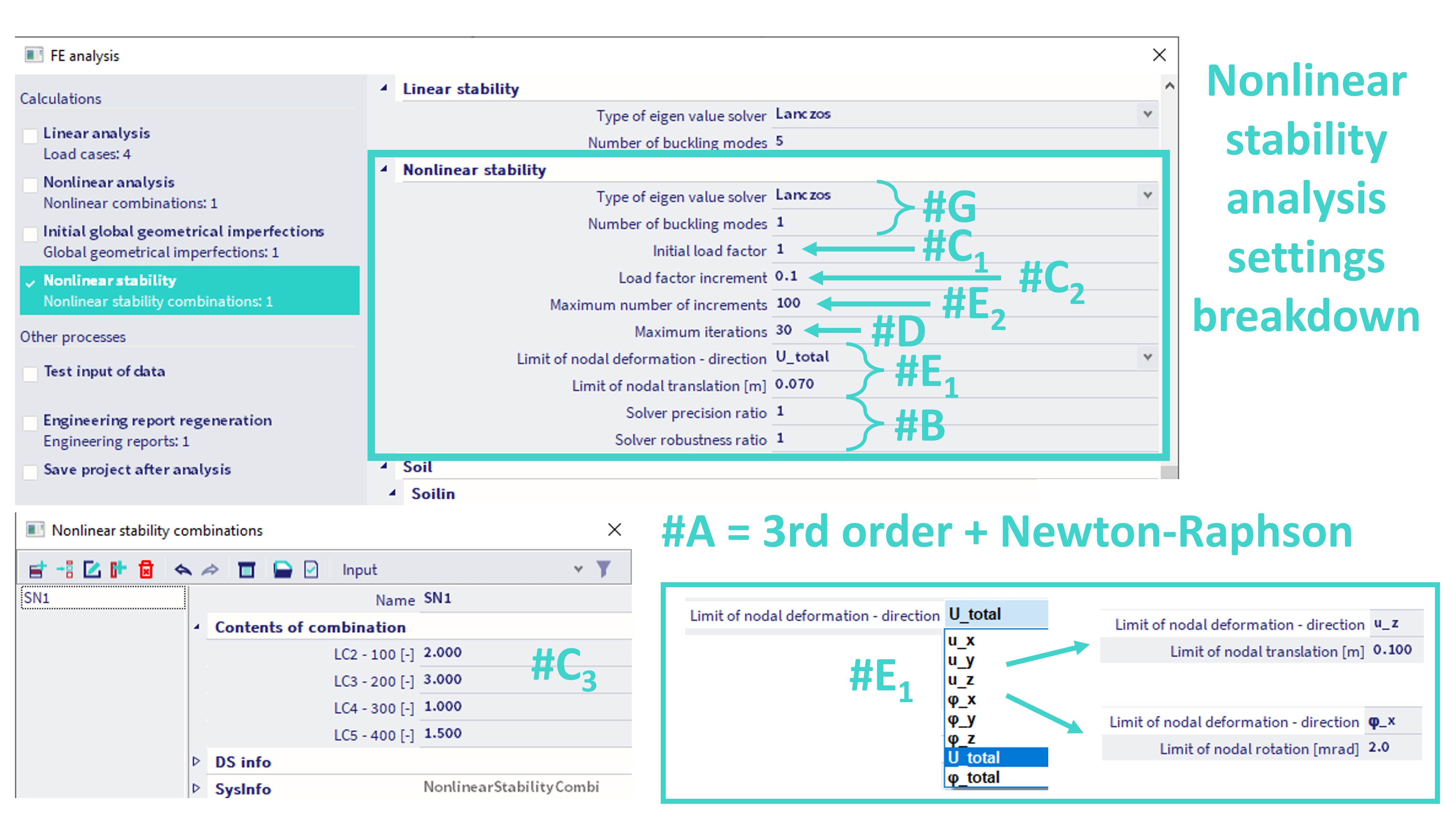
#A = For nonlinear stability, the 3rd order (large deformations) along with Newton-Raphson method are always used, hence this setting is not possible to be altered.
#B = Solver precision and Solver robustness ratio = the same as in case of nonlinear analysis, but applied only for nonlinear stability calculations
#C1 = Initial load factor (default value is 1) = this is portion of the NL.ST.C. content, which is applied in the first increment of the nonlinear stability analysis process.
#C2 = Load factor increment (default value is 0.1) = this is portion of the NL.ST.C. content, which is being added in each subsequent increment during the nonlinear stability analysis process.
#C3 = Content of the NL.ST.C - the whole content is being added - e.g. if there is load case of self-weight and some different load case with force loads, during the increments, both loads (self-weight and force load) are being added by the same ratio (hence also self-weight is being added over 100%).
#D = Maximum iterations = maximal number of iterations within each increment, the same as in case of nonlinear analysis,
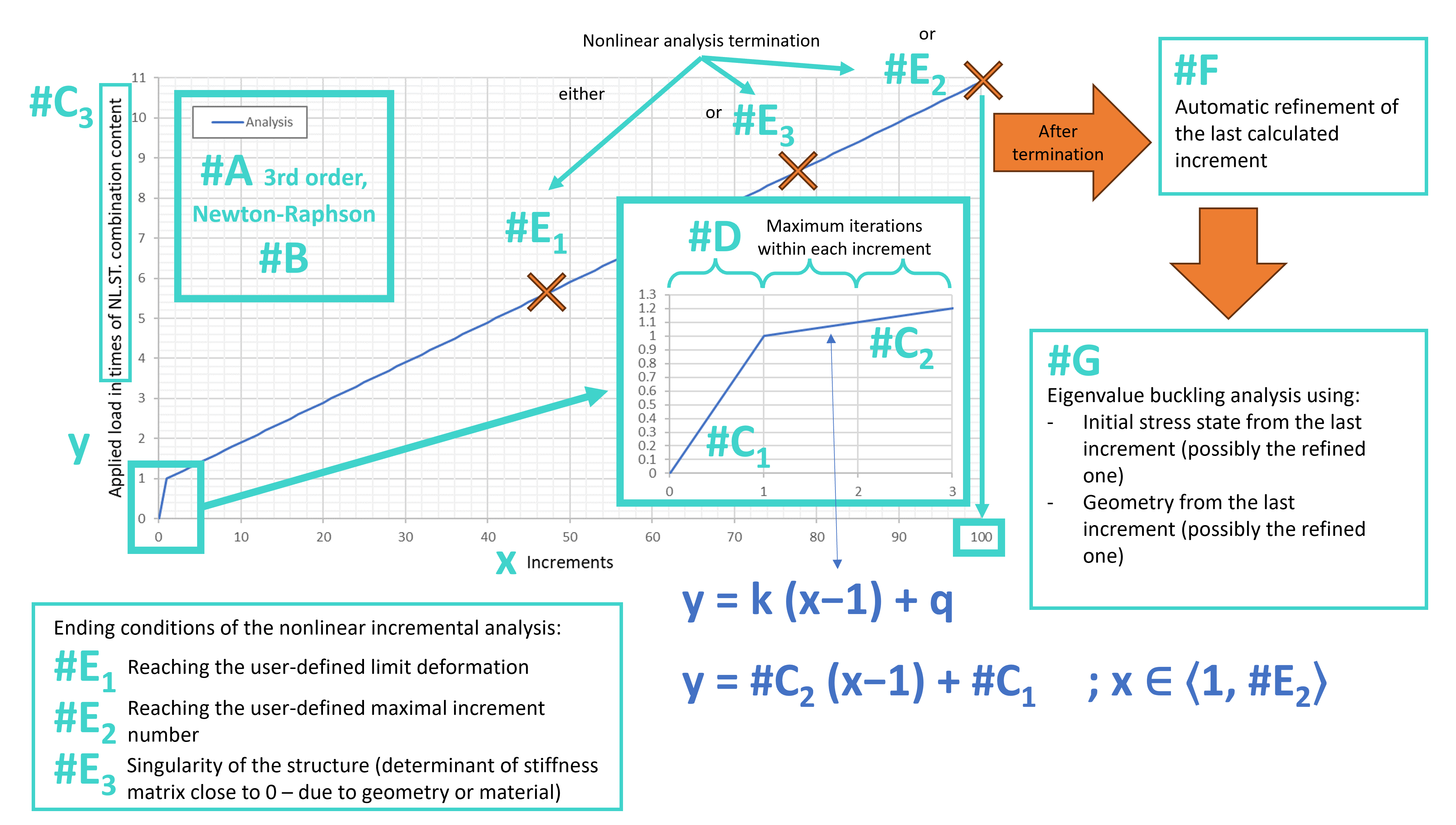
As mentioned before, the nonlinear analysis in the background of the nonlinear stability analysis process is being calculated until one of the ending conditions is achieved. There are in basic three ending conditions #E1 - #E3 explained in detail below:
#E1 = The last increment is the one, where user defined limit deformation is reached. It is possible to define the type (direction) of this nodal deformation, where 3 translational directions and 3 rotational directions are available to be selected. Also, total translation and total rotation, which is vector sum of the corresponding entity might be selected. The corresponding limit value for the selected deformation is the defined, in units of length if the deformation is of translation type, or in radians is the deformation is of rotational type. This user defined limit is then checked in each increment of the analysis, and the maximum of all the nodes is evaluated for the ending condition.
#E2 = The user might explicitly define the number of increments of this process (the default is 100). The nonlinear analysis running will be ended upon reaching this increment number. This might be used in order to define what exact load should be used for the subsequent eigenvalue analysis - e.g. in the presented case, with initial load factor of 1 and load factor increment 0.1 and maximum 100 increments, the maximal load would be 1+0.1*99, hence, 10.9 times the content of the NL.ST.C. (if the other ending conditions are not achieved before this amount of load is applied). It is also possible to check the number of last increment in the LOG file of the corresponding analysis in the TEMP folder (see in the next chapter below). Alternatively, this might be used to limit the analysis, so the calculation takes less time in total.
#E3 = The analysis might end due to reaching singularity, hence if the determinant of either the stiffness matrix is reaching 0, due to either large geometrical displacements, or material yielding.
#F = After one of above mentioned ending conditions #E1 or #E3is achieved, the last increment is refined, hence, the analysis process returns one step back and the application of the load in the last increment is refined, in order to achieve more precise result. The refinement factor is 10 (not possible to alter by user), hence, 10-times more finer then the load factor increment. In this example case, it means 0.01 (0.1 / 10), hence 1% of load will be added in each refined increment.
#G = Considering the geometry and stress state from the last increment of previous process, the eigenvalue analysis is conducted. Type of eigenvalue solver might be selected, and the number of buckling modes, analogical to the settings of the linear stability analysis.
The whole process is explained graphically in the figure and graph below, where on the x-axis there is number of increment, and y-axis the applied load (in times of NL.ST.C. content):
Where to check the increment number, and data for graph convergence
In order to check what is the reason of the nonlinear combination termination which precedes the eigenvalue buckling within the nonlinear stability analysis, it is possible to check the LOG file of the corresponding analysis, as depicted in the figure below. It is necessary to locate the corresponding sub folder within the TEMP content of the calculated *.esa file (see the figure below).

For example in this case, the limit of maximum number of increments, #E2, is 3., and limit of deformation ,#E1, is 1 meter (total deformations of all the nodes are checked, the largest one is evaluated for this criterion). In the LOG file, the last increment (INCR) is increment number 3, afterwards the analysis is terminated. Hence, the ending condition #E2 has most likely been achieved (unless the both conditions would be achieved simultaneously in the same increment, what however might be checked running the analysis again with larger increment number, or different deformation limit).
Also, the maximal displacements (translation and rotation) of the node with the maximal value might be checked in the corresponding $001$064.GRF4000001 file located in the corresponding folder, which is a text file with data for the convergence graph. The content is depicted in the figure below. We can see that the 12th step (considered cumulatively), what is the 3rd increment, 4th iteration, the maximal displacement was 8.144368 mm in the node number 100 (FEM node), and maximal rotation was 0.8018183 mrad in the node number 47. The total applied load was equal to 120%, what corresponds with the analysis settings (initial load factor = 1, load factor increment 0.1, total 3 increments, hence 1+0.1*2 = 1.2 ... 120%).
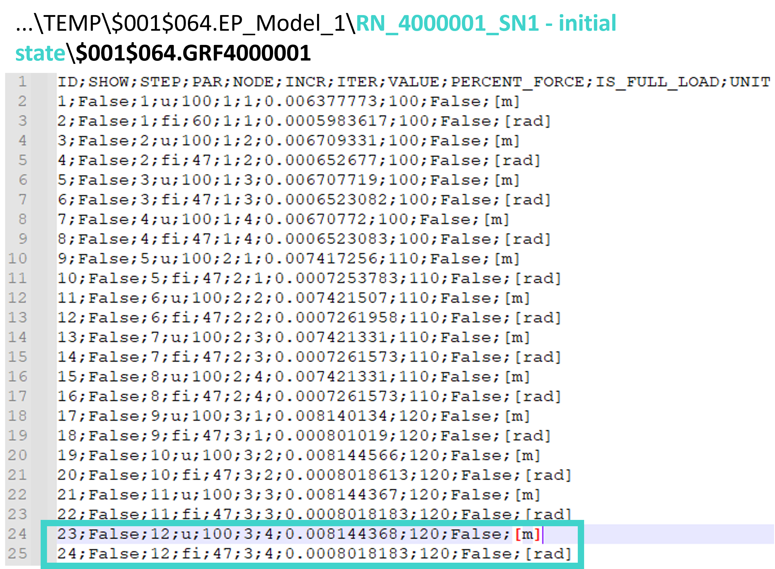
Note: analogically, these data might be found for nonlinear analysis, in sub folders corresponding to nonlinear combinations if applicable for the project.