Soil pressure and water pressure

Several types of load (point force, line load and surface load) can be defined as what is called "soil pressure" or "water pressure ". Both loads are quite related and will be explained together.

Both load types appear only if a structure is located underground.

$image\soilload1.gif$

The pressure is generated on the basis of data provided in the dialogue. It means that the "geologic" data are derived exclusively from the borehole profile provided. The generated soil pressure takes no account of possibly displayed earth surface. Even if the surface has been calculated and is displayed, the program does not calculate the intersection of the surface with the member that is subject to the soil pressure. The part of the member that is underground is determined only and solely from the specified single borehole profile. See the picture below.

$image\soilload3.gif$

There are three columns defined. There are several boreholes defined. The surface was calculated and is shown in the picture – the inclined line joining the top ends of the two boreholes. The soil pressure was input on all the columns. The left most borehole was used as the reference parameter for the definition of all three loads. That is the reason why the distribution of the soil pressure generated on all columns is identical. In other words, the two columns on the right are subject to soil pressure even above the surface. The calculated surface does not influence the generation of the soil pressure.

In depth h (point a), the intensities of the generated loads are:

SigV,a

If a is located above water level

(h <= H’d), then (h * Gdry)

If a is located below water level

(h > H’d), then (H’d * Gdry + H’w * Gwet)

It works ONLY in the negative direction of global Z-axis!

SigH,a

SigH,a = SigV,a * k0

SigW,a

If a is located above water level

(h <= H’d), then ( 0)

If a is located below water level

(h > H’d), then (H’w * Gwater)

This would lead to a distributed load as in the image below:

$image\soilload2.gif$

Water and soil loads can be input for the following load cases:

action type = "permanent" and load type = "standard",
action type = "variable" and load type = "static".

The procedure to input soil / water pressure

Open service Load.
Start function the required load type (point, line, surface).
Adjust the parameters - see below.
Confirm with [OK].
Apply the load on required entities.

Soil / water load parameters

In addition to common parameters for point, line and slab load, this load type requires the input of the following data:

Type	Must be set to Soil pressure or Water pressure.
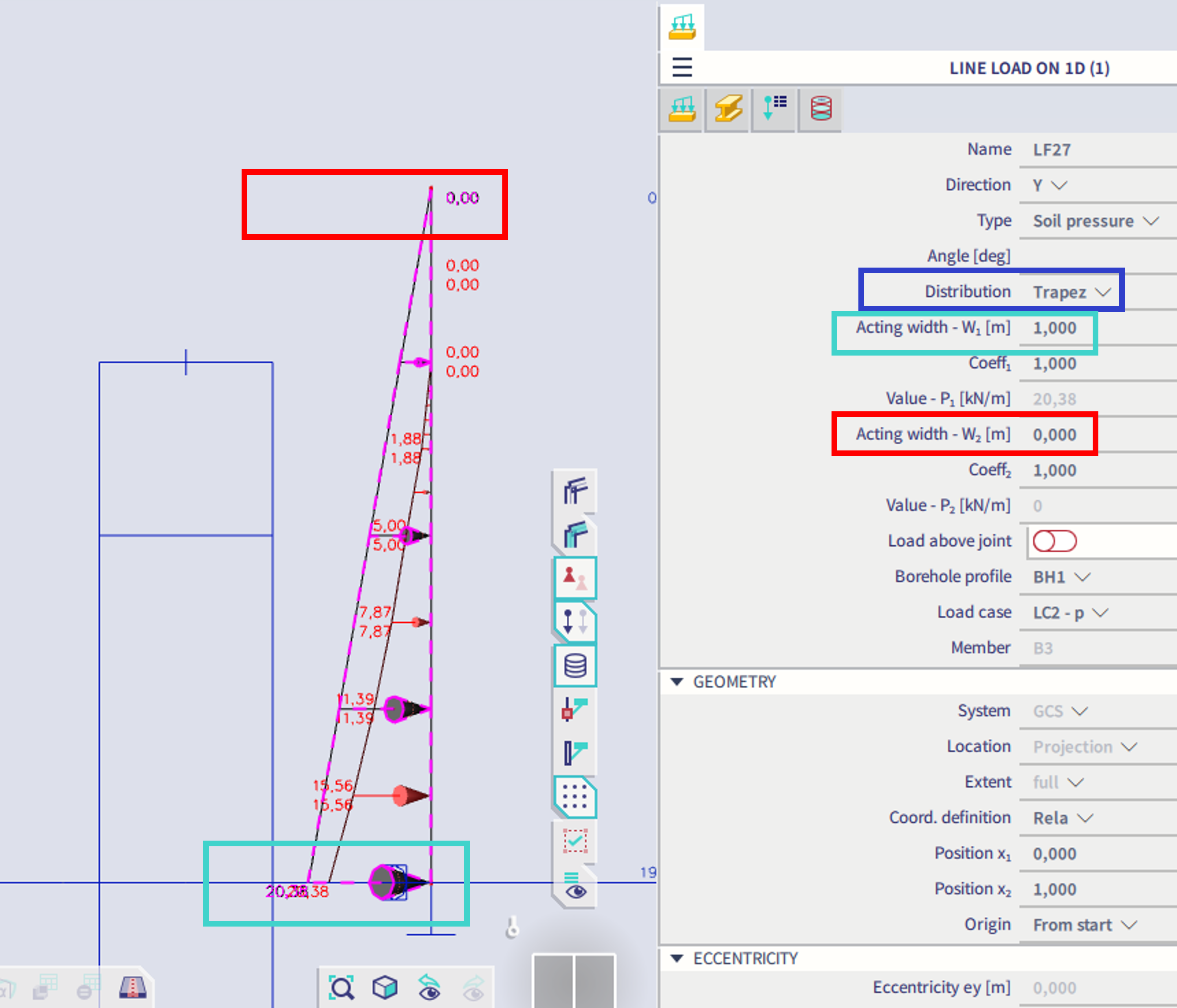
Distribution	Only for line load. The line load may be uniform or trapezoidal.
Acting area	Only for point load. Defines the acting area for the load.
Acting width	Only for line load. Defines the acting width for the load.
Coefficient	Multiplies the pressure.
Borehole profile	Specifies the borehole that is used for the generation of the pressure.

The soil / water pressure is displayed as shown in the picture below.

The brown diagram represents the "defined" load. It has been defined along the whole column.

The green diagram represents the "generated" part. The generated soil pressure reaches just to then top of the borehole (that was used as the reference borehole).

The calculation considers the green, i.e. generated, load.

$image\soilload4.gif$

Note: Water pressure is generated only below the level of underground water. If the whole model is above the water level, no pressure is generated at all.

Features and behaviour

Line load

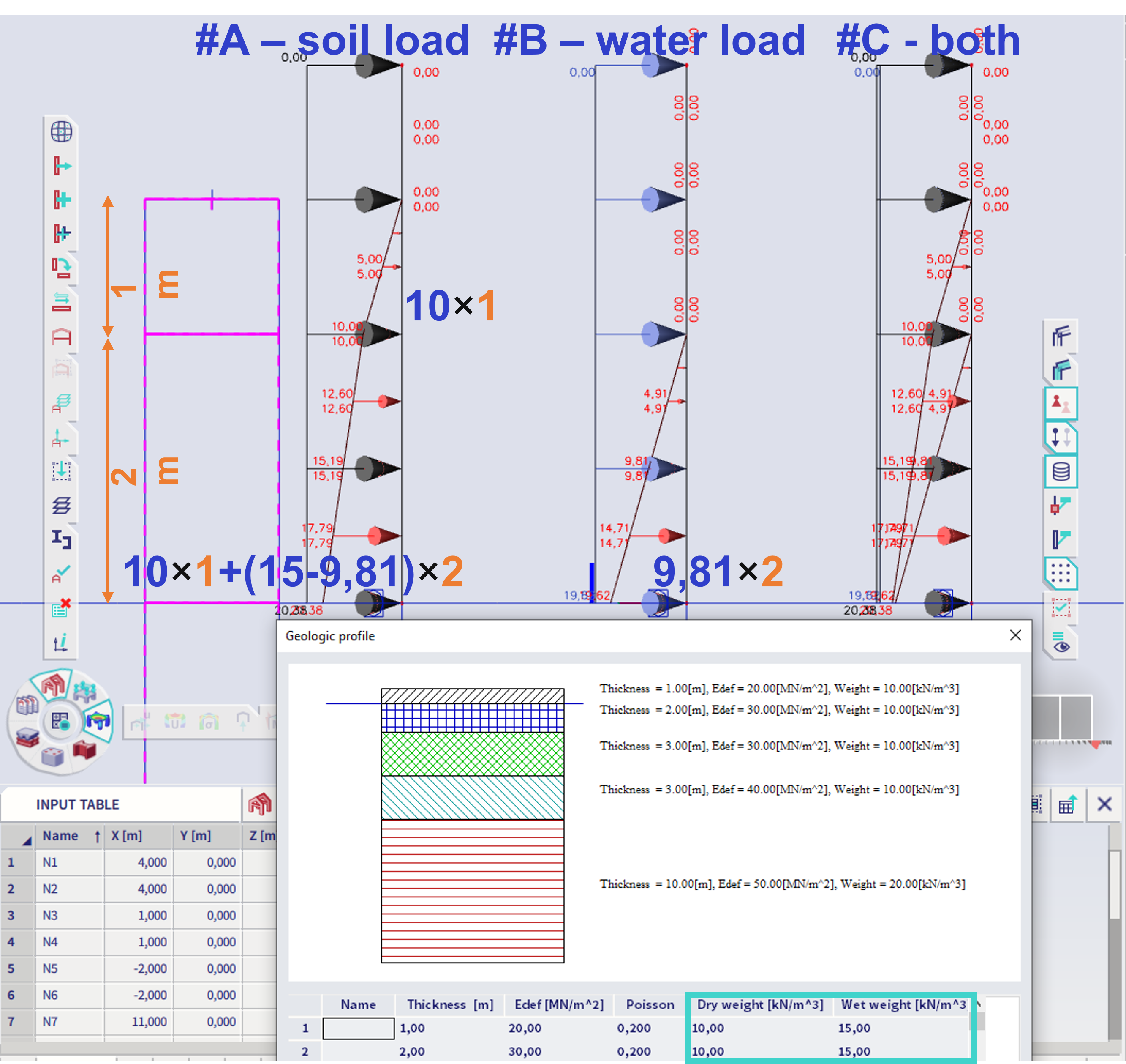
In example below, there are three cases:

#A = only soil load; #A = only water load; #C = soil load and water load

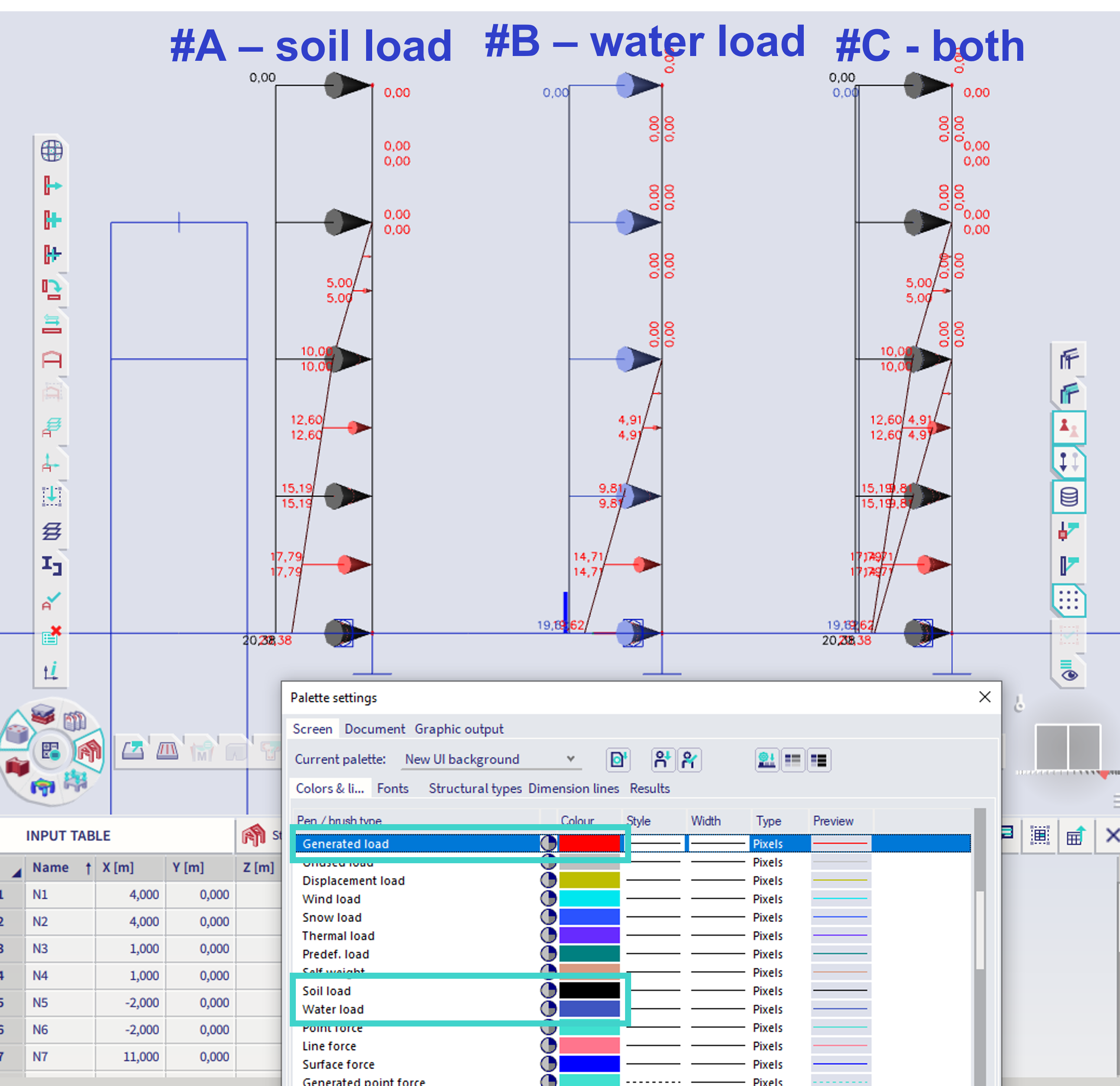
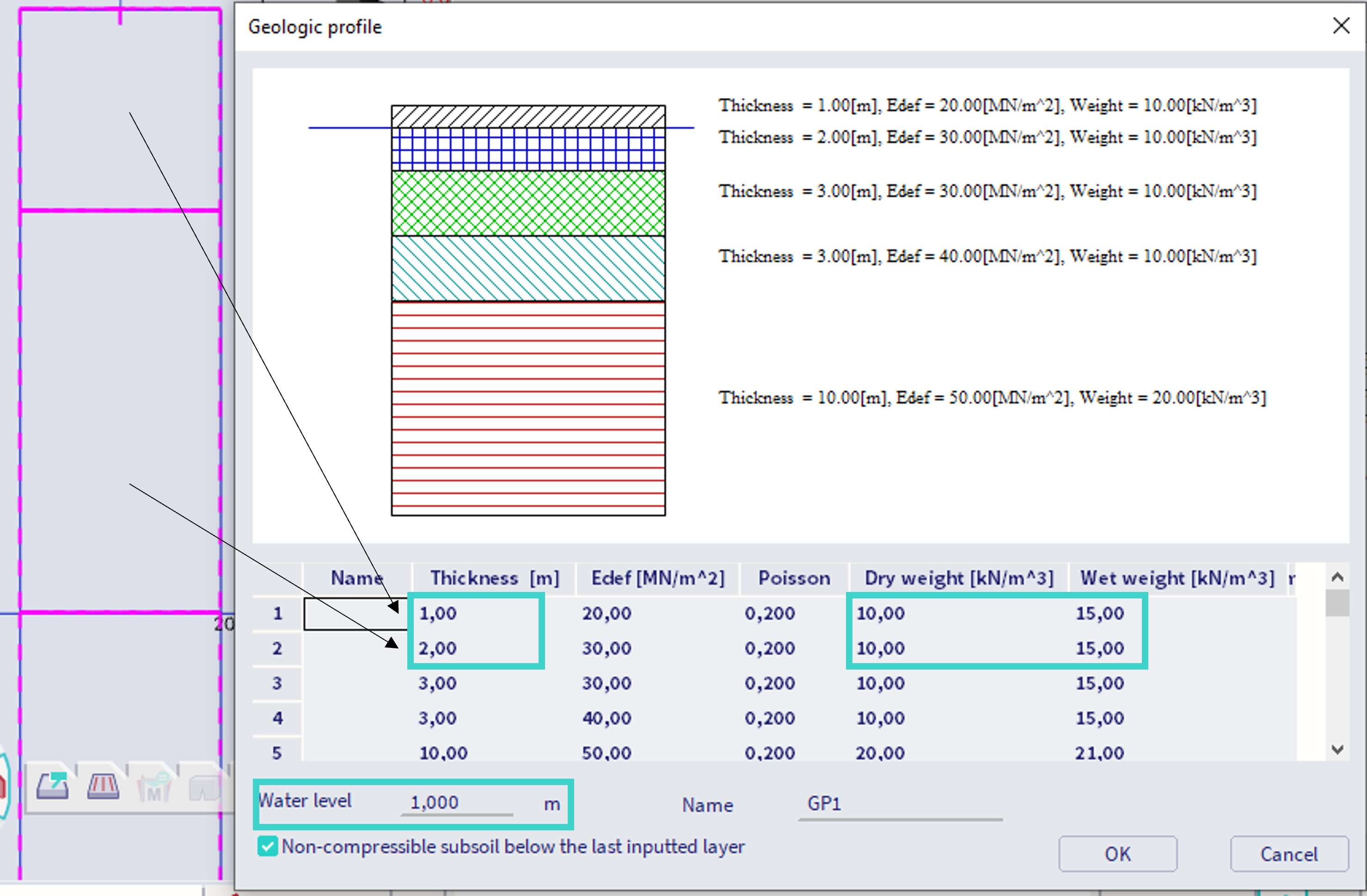
The borehole profile is as below. Only the first two soils are applied now. Water level is in 1 m.

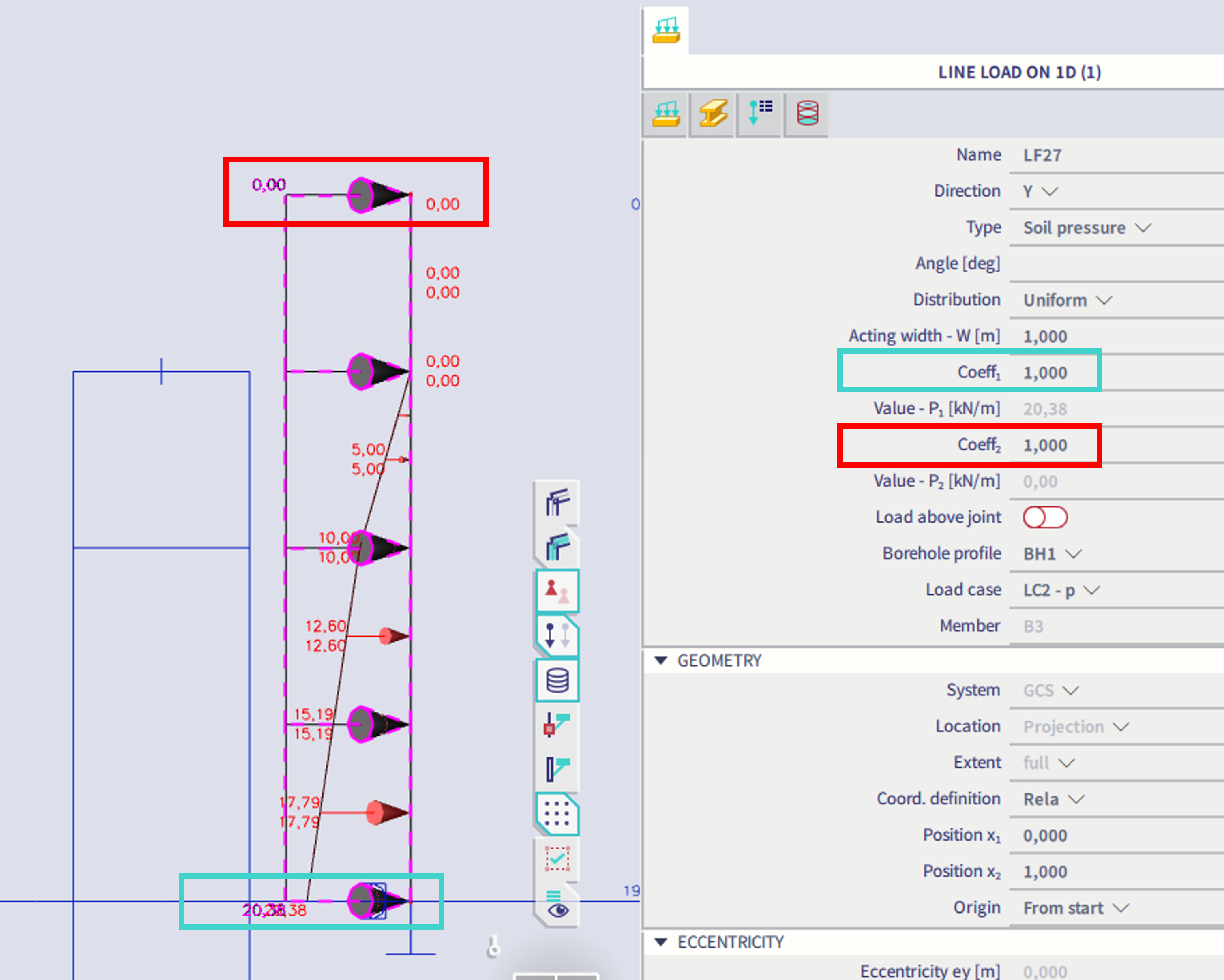
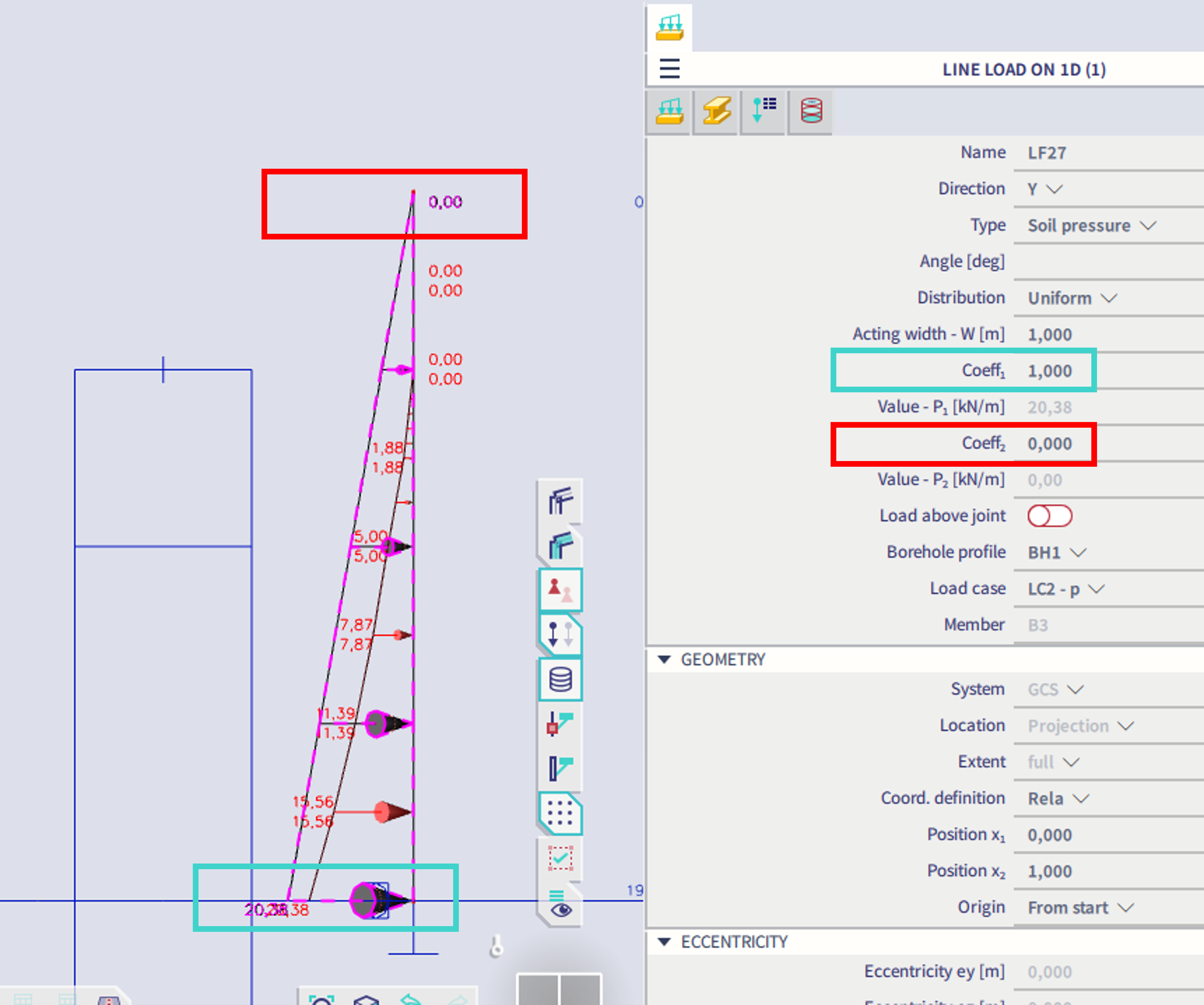
It is possible to alter the coefficient which specify the ration between the vertical and horizontal load, in the top and bottom position of the line load, noted Coeff1 and Coeff2. It is not possible to alter this coefficient for each soil separately, only for the whole line load (all soils at once). If the values at the ends are different, the values in between are linearly interpolated.

It is possible to alter the acting width - at the top and bottom of the soil-line load itself. The values between are interpolated.

A little check of expected loads:

Surface load

In case there is a soil load applied on a 2D surface, e.g. wall, and there are only walls in the current selection, user can see the surface load graphically plotted by area with arrows:

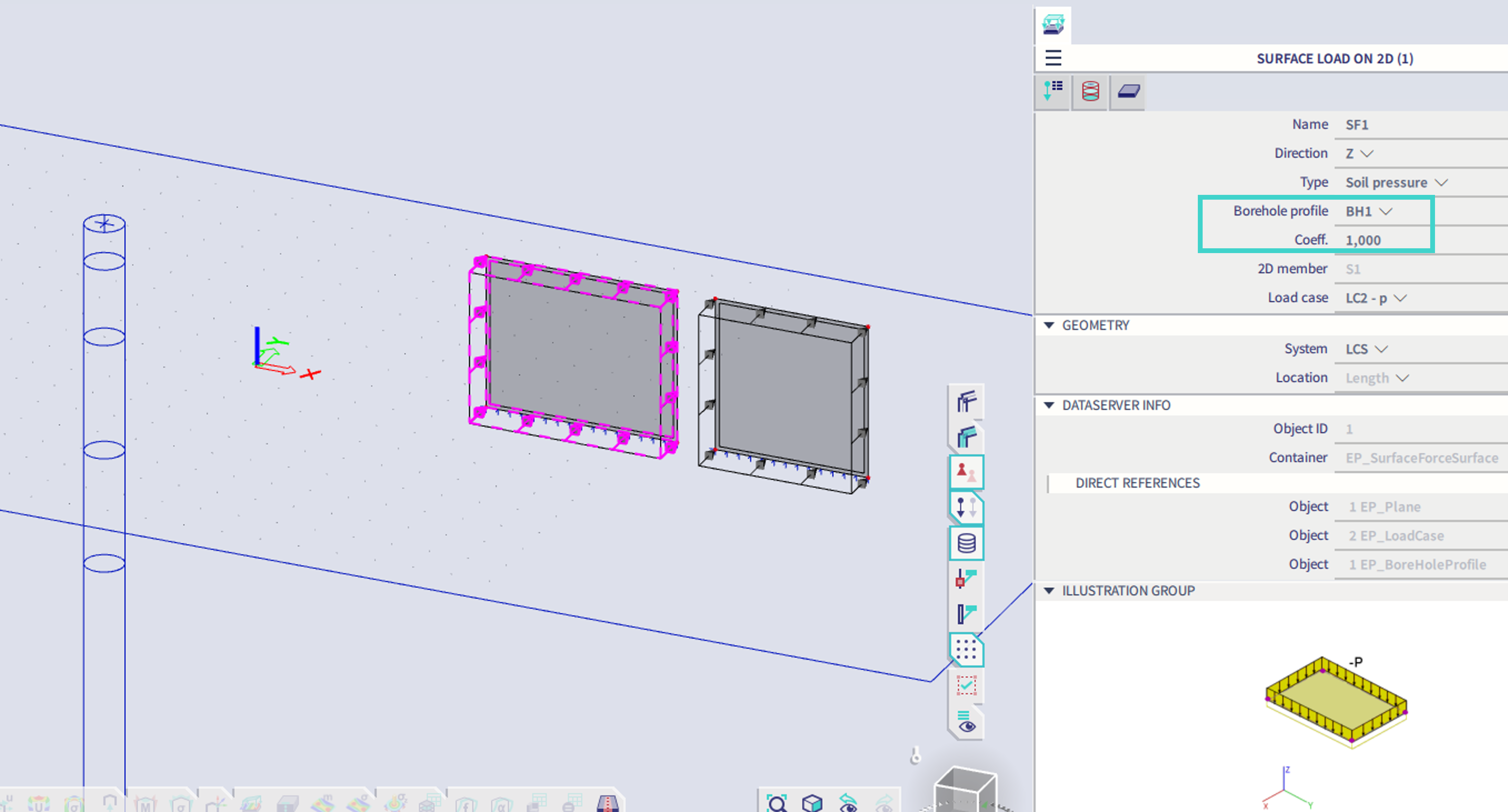
However, in case also 1D members are in the selection, the 2D surface load applied on a 2D surface of a certain shape (rectangle in case below) is visible only as offset of this shape (inner rectangular frame in case below), because the unit of this surface load is the coefficient value, so it is not in match with the unit of the line load (kN/m):

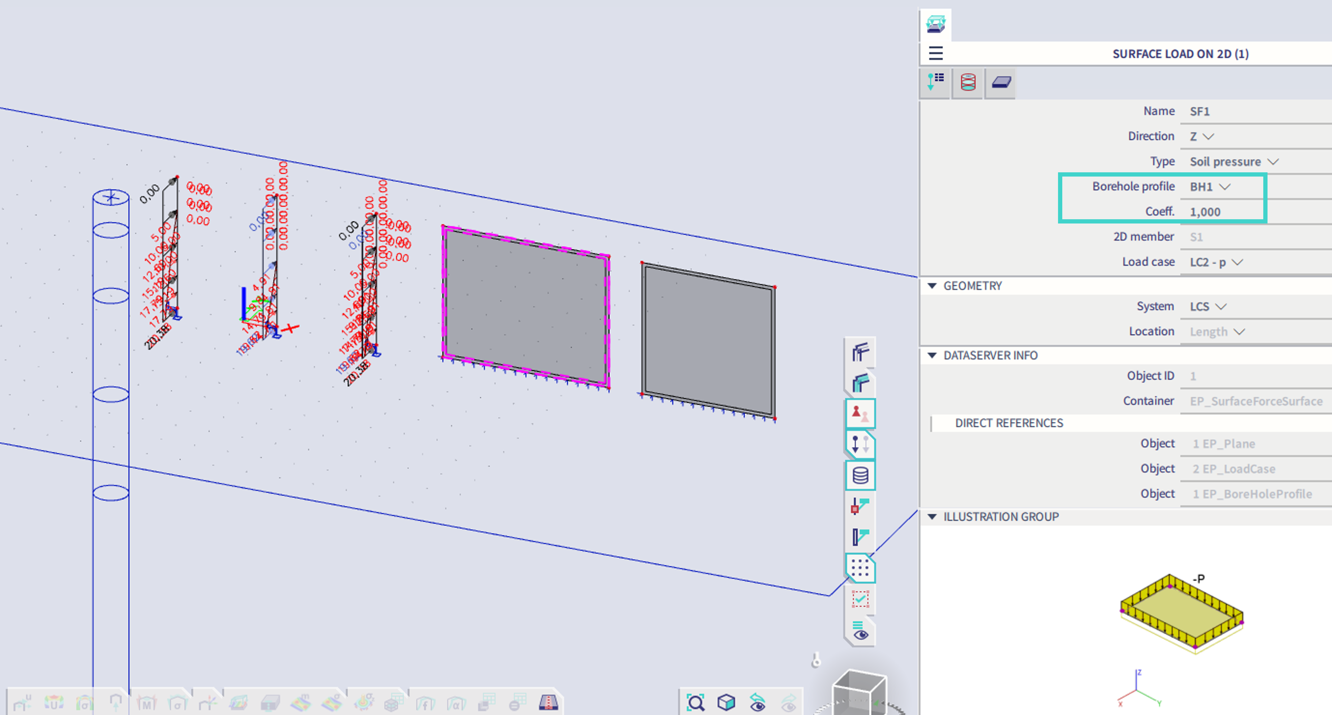
The generated load is not visible directly, but the feature of 2D surface loads might be utilized in order to see the applied load:

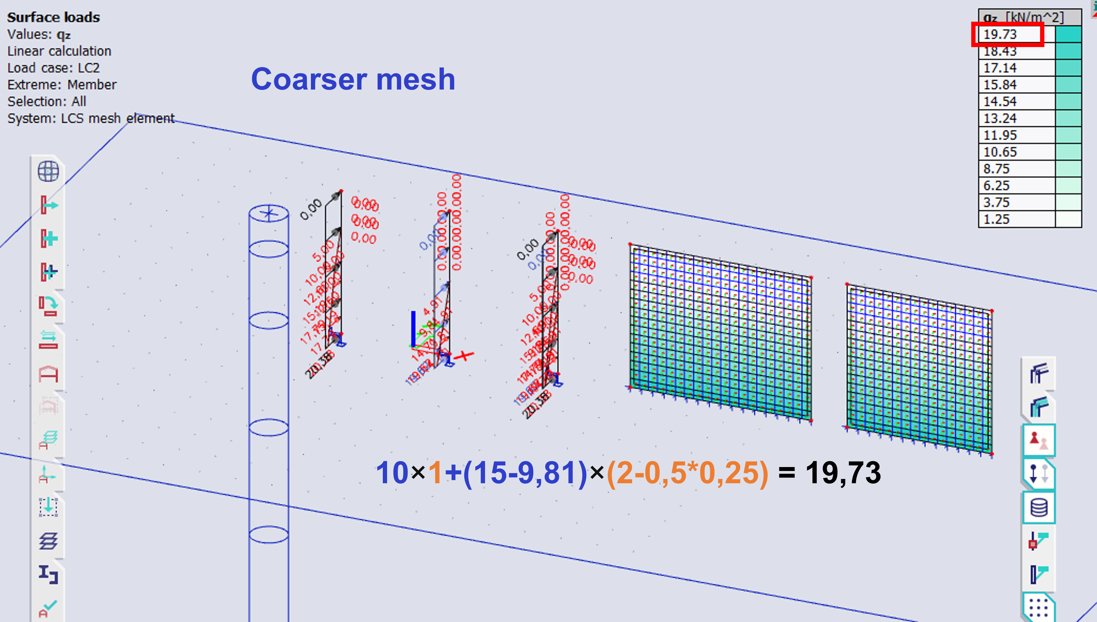
Utilizing this feature, the load value in the centre of gravity of the finite elements is plotted. If finer mesh is applied, the value is slightly different (but the resultant of the corresponding reaction is the same):