Displaying the results in selected sections

1D member

By default any result diagram is displayed in all calculated sections. If required, it is however possible to limit the diagram to a limited set of explicitly defined points – user defined sections.

Whenever a function displaying some result quantity is started, the parameters controlling the behaviour of this function are displayed in the Property window. One of the parameters is called Section. The meaning and consequences of this parameter will be demonstrated on a simple continuous beam.

Let’s assume a simple three-span continuous beam subject to uniformly distributed load. The beam is defined as a set of three beams attached to each other.

Further, let’s define one section in the middle of each span.

Finally, let’s display the diagram of calculated bending moment My. Using the default setting (parameters Section set to Ends), the diagram may look like:

Now, let’s change the setting of parameter Section to Ends. The calculated values of bending moment will be drawn in end points of each defined beam.

Now, let’s change the setting of parameter Section to Input+Ends. The calculated values of bending moment will be drawn in end points of each defined beam and in three defined sections.

Now, let’s change the setting of parameter Section to Input. The calculated values of bending moment will be drawn only in the defined sections.

Slab

By default any result diagram is displayed by means of isolines / isobands. If required, it is however possible to limit the display to a diagram along a defined section – user defined sections.

Whenever a function displaying some result quantity on slabs is started, the parameters controlling the behaviour of this function are displayed in the Property window. One of the parameters is called Drawing. The meaning and consequences of this parameter will be demonstrated on a simple slab.

Let’s define a rectangular slab subject to any load.

Further, let’s define a section cutting the section e.g. in the middle.

Let’s calculate the slab and display e.g. internal forces.

Let’s try all the options for the Drawing parameter.

Standard	The results are shown using isolines/isobands. A legend is displayed in the top right corner of the graphical window.
Section	The results are drawn along the defined section across the slab. Function Setup > Scales can be used o control the size of the diagram.
Resultant	The resultant along the section is calculated. Again, function Setup > Scales can be used o control the size of the diagram.
Standard + Section	Options Standard and Section are cmbined together.
Trajetories	This option works for principal quantities only. The direction (trajectory) of the quantity is shown. A legend is displayed in the top right corner of the graphical window.

Type of diagram in the section

According to the needs of a particular calculation, SCIA Engineer allows you to select the most appropriate type of representation of the result in a section across the slab.

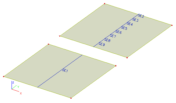
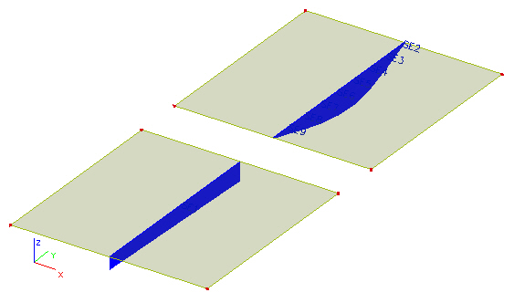
To understand more the individual options, let us input two identical slabs subjected to the identical load. Further, let us define a section across each of the slabs. The first slab has one section defined across the whole width. In the second slab, let us divide the section into eight intervals to have finer results - see the image below.

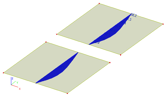
Precise

The precise distribution of the displayed result quantity is draw along the section.

In our example of two identical slabs, diagrams on both slabs look identical as well.

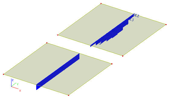
Uniform

The average value of the result is displayed.

This option may be useful to see the effect of the structure and loads to the particular section.

The example of two identical slabs produces the following results. The "precise" area must be equal to the area of the "uniform" rectangular diagram.

Trapezoid

The distribution of the quantity along the section is approximated by a trapezoid.

This option may be useful if you model your structure in parts and use the reactions of upper parts as load for lower parts. It may be practical to idealise the effect of the upper part by this trapezoidal distribution.

 

The example of two identical slabs produces results where the force resultant and moment resultant of the trapezoidal diagram are equal to the resultants determined from the "precise" diagram.

Procedure to select the type of diagram in the section across a slab

1. Have the project calculated.

2. Open service Results.

3. Call a function that displays the results in slabs in sections, i.e.:

   1. 2D members > Deformation of nodes,

   2. 2D members > Member 2D – Internal forces,

   3. 2D members > Member 2D – Stresses.

4. Note that there are two items named Drawing in the property window – on condition that the first Drawing is set to Section (otherwise there is just one Drawing item in the property window).

5. Set the first Drawing to Section.

6. Set the second Drawing to the required type of diagram (Precise, Uniform, Trapezoid).

7. Select the quantity to be displayed.

8. If required, adjust other display parameters.

9. Refresh the screen.

Examples of diagrams in sections

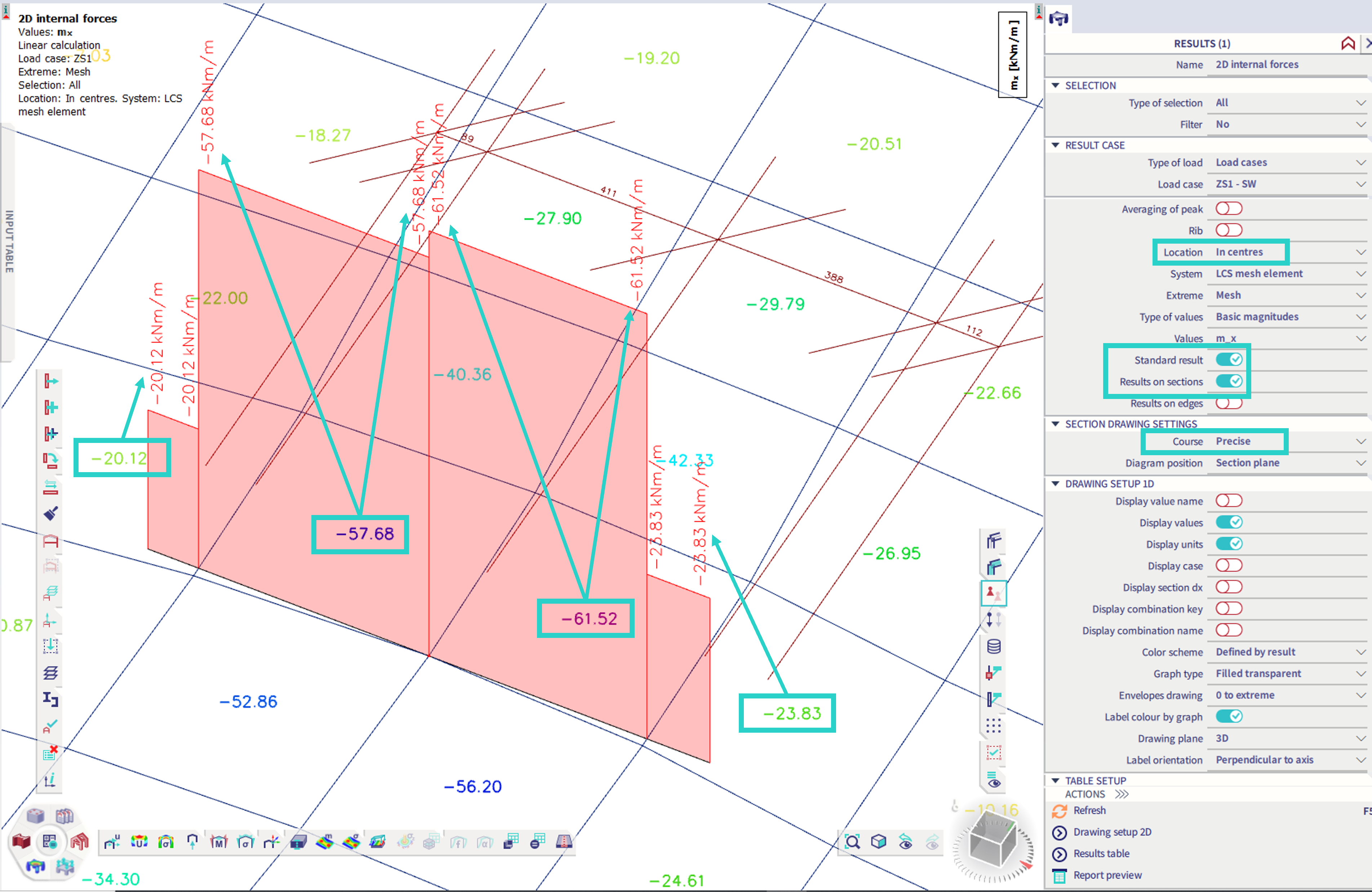
An example of a 2D result (mx) and a section is provided below.

For location "in centres", the results of section for precise, average and trapezoid courses is provided . The precise course considers the averaged values of the finite elements, the average respects the same area of the graph, and trapezoid is based on least square method (but utilizing discrete values, hence it might lead to smaller values then averaged)

For location "in nodes averaged", the results of section for precise, average and trapezoid courses is provided . The results in this case are analogical to the previous case.

The other two locations ("in nodes no average", and "in nodes averaged on macros") are considered in a similar manner.

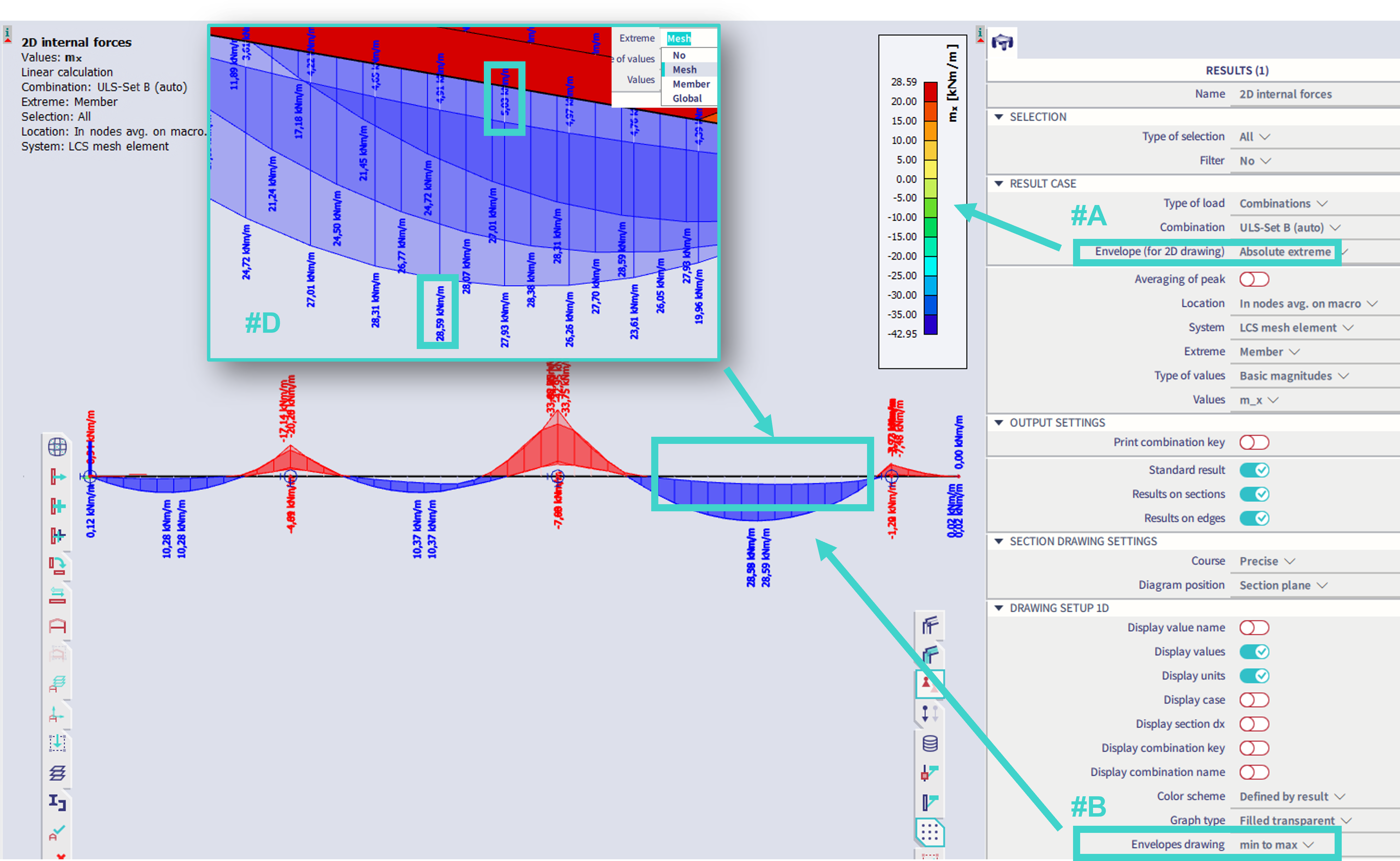
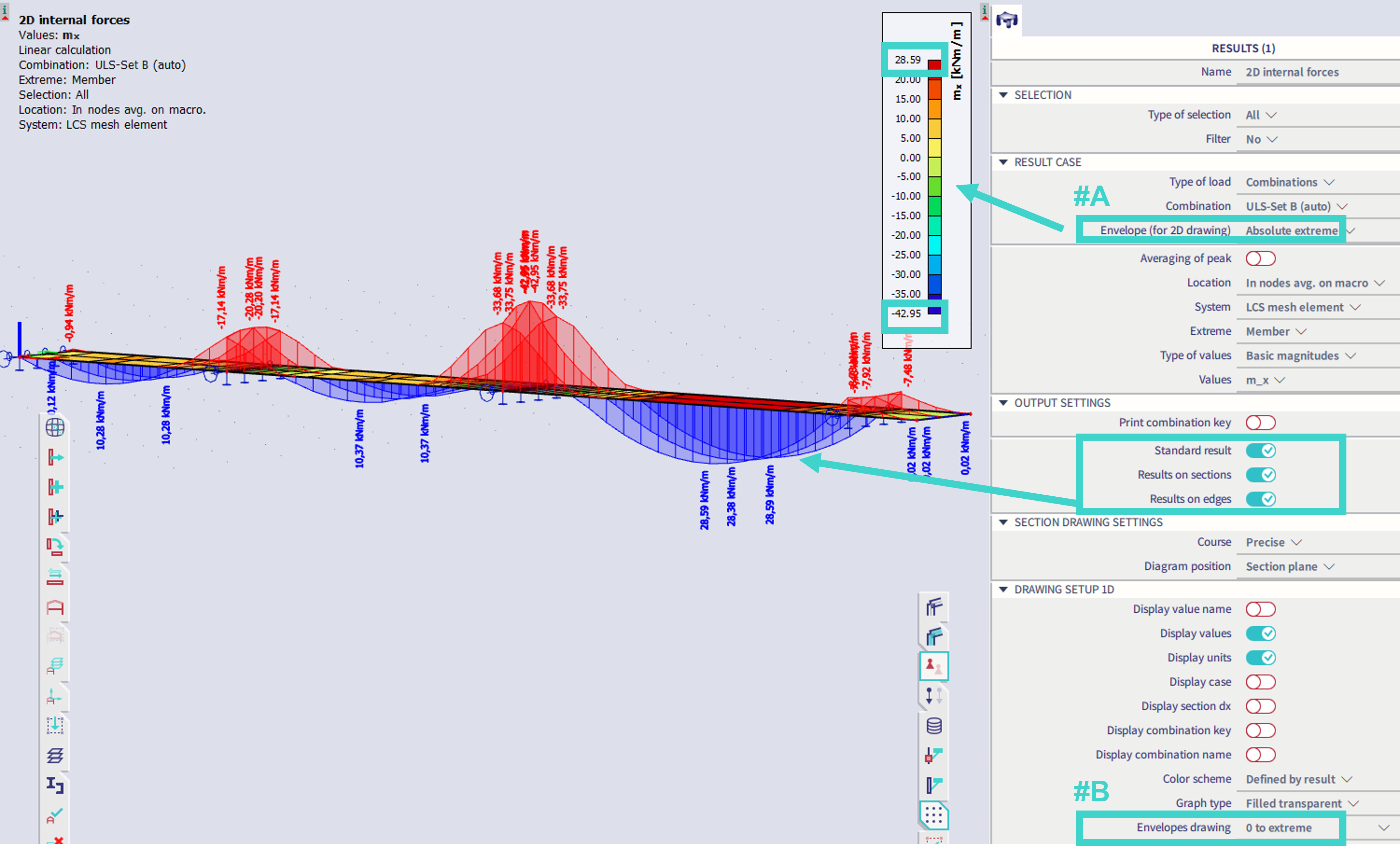
Results 2D - Results on sections, Results on edges - Combinations, envelope - properties

For 2D results (e.g. 2D internal forces), following options are possible to be graphically plotted: Standard result (on 2D members by colour-scale); Result on sections; Result on edges.

For the result case "combinations", options for Envelope drawing: "Minimum", "Maximum" and "Absolute extreme" are available.

The option "Minimum" (#A in figure below) shows the minimal values (mathematically) from the selected combination (respecting the linear combinations within the selected envelope combination). The property "Envelope drawing" (#B in figure below) has no meaning in this case, as only the minimal values are plotted.

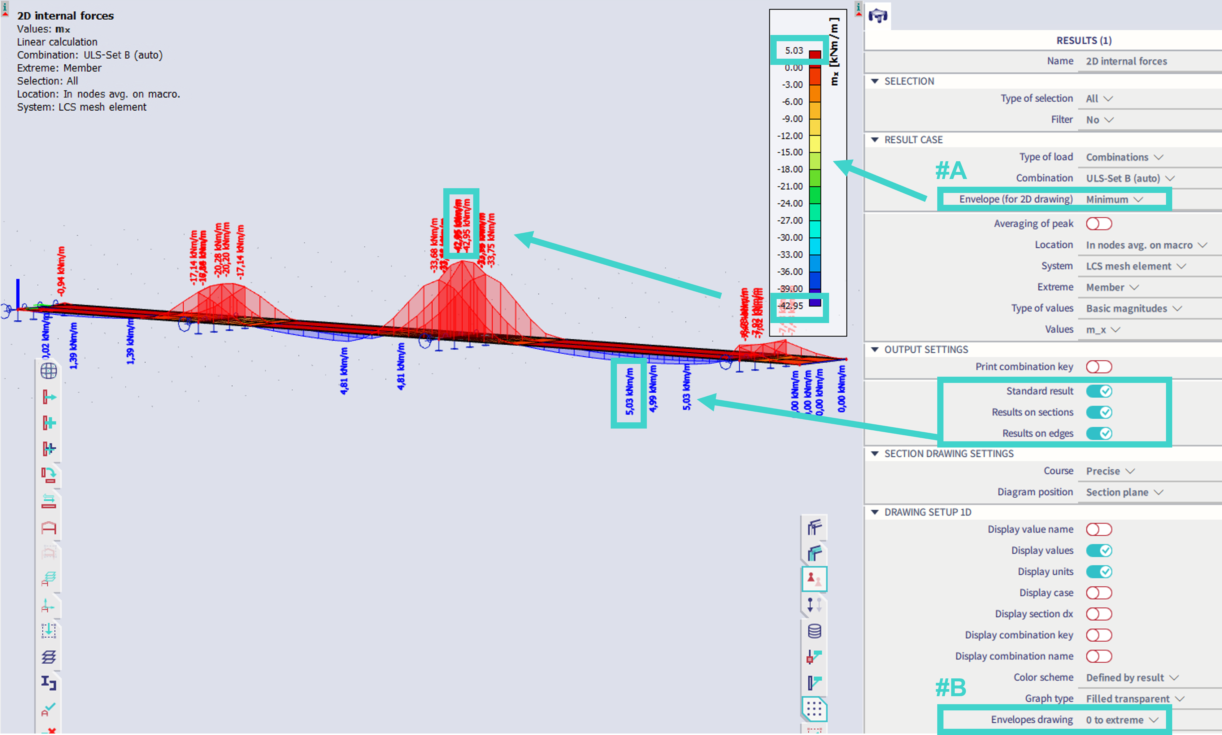
Analogically, the option "Maximum" (#A in figure below) shows the maximal values (mathematically) from the selected combination (respecting the linear combinations within the selected envelope combination). The property "Envelope drawing" (#B in figure below) still has no meaning in this case, as only the maximal values are plotted.

If it is desired to see, from which exact combination (e.g. linear combination within the envelope combination) the value is obtained, the properties to display combination key and name needs to be turned on (#C in figure below).

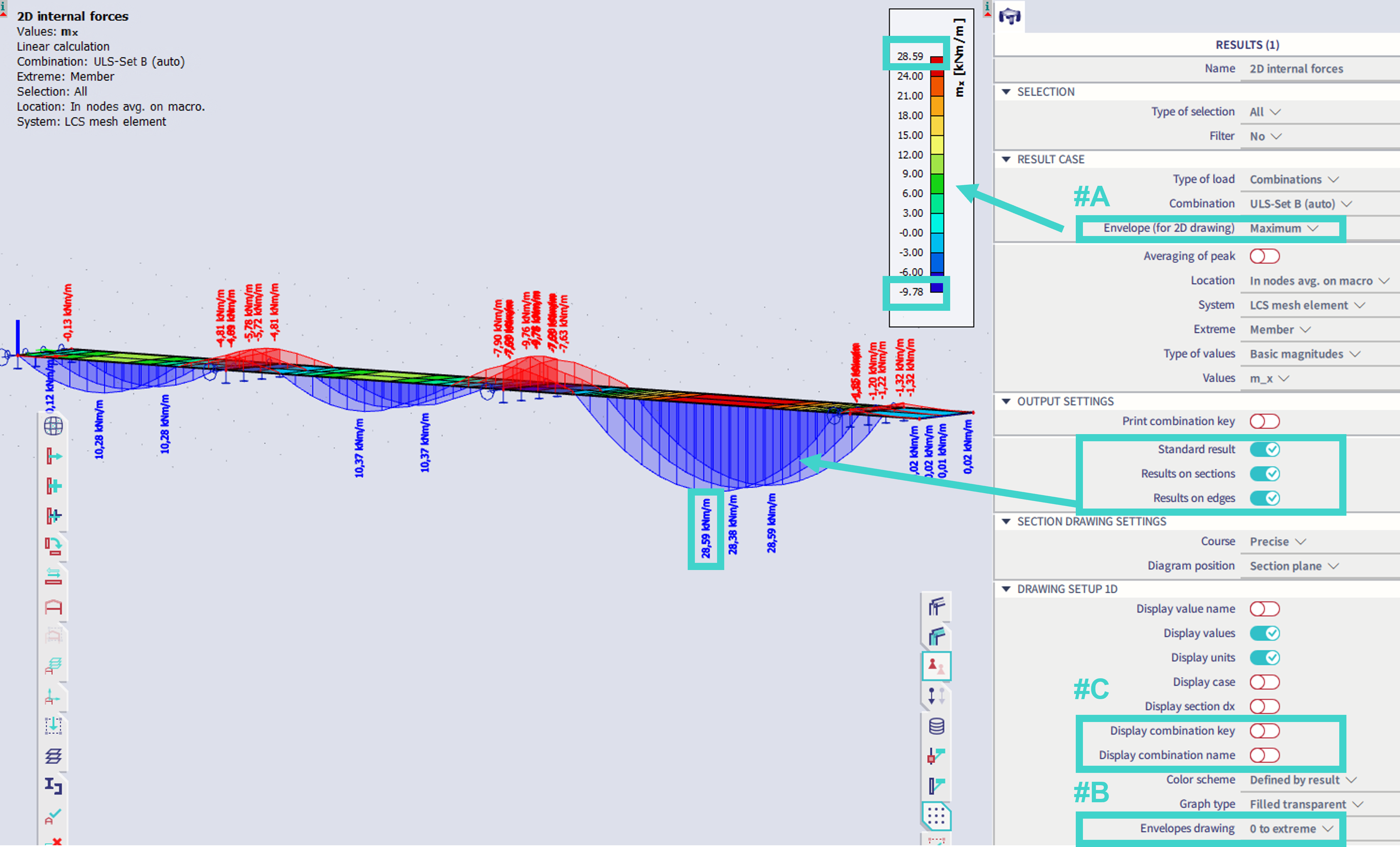
The option of "Absolute extreme" (#A in figure below), shows the envelope of the current combination (minimal and maximal values in one graph). The option of envelope drawing "0 to extreme" (#B in figure below) provides the graphical plot of the selected values aligned up to the corresponding axis (section or edge axis).

Changing the option to "min to max" (#B in figure below) plots the graph within the minimal and maximal values in the current section. Both values (min and max) could be graphically depicted if the "Extreme" property is switched from "member" to "Mesh" (#D in figure below).