Design of cable members
Definition, application
Cable is a special type of beam local nonlinearity, which can be applied on 1D member in model. Cable members possess only axial stiffness (in tension only), the bending stiffness is zero (resulting in 0 values of internal forces Mx, My, Mz, Vy, Vz). In order to implement this feature, a geometrically nonlinear analysis (3rd order, Newton-Raphson) needs to be calculated, therefore it is necessary to perform the" Nonlinear calculation".
Modelling
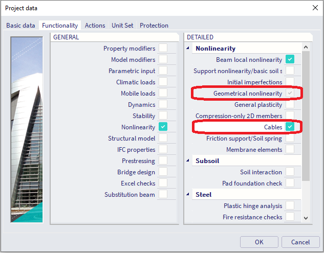
In project data, the functionality "Solver settings" must be on, along with detailed functionalities: Beam local nonlinearity, Geometrical nonlinearity and Cables (turning on the functionality Cables automatically turns on the Geometrical nonlinearity). See the picture below.
In order to define a cable, assign the Nonlinearity 1D attribute
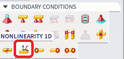
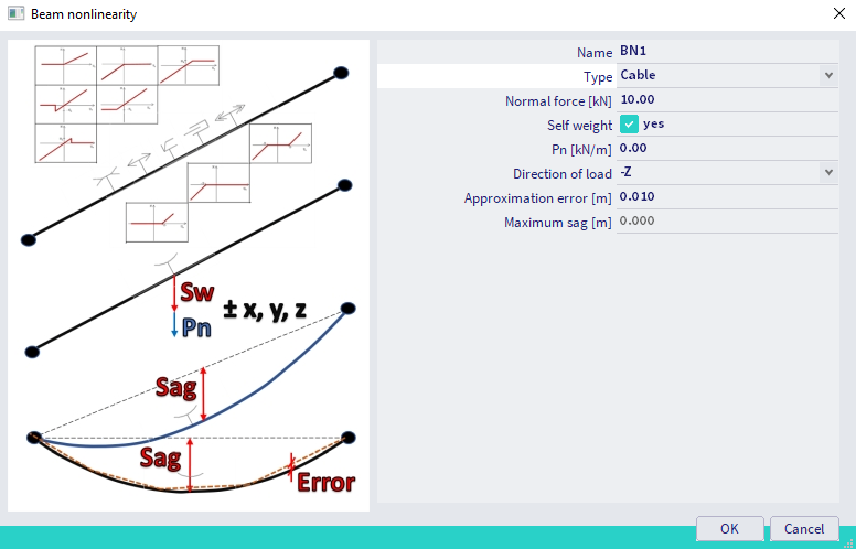
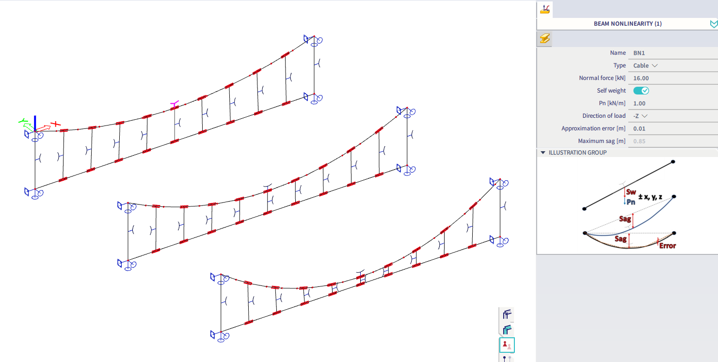
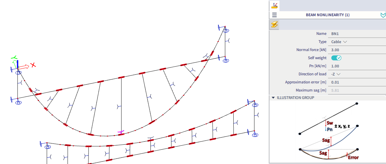
to a chosen beam member, select the Type Cable:
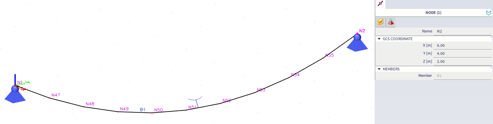
When attributed to a certain 1D member, the shape of that member changes from straight line to a catenary curve (more precisely a linear approximation of a catenary curve). Such 1D member is also marked by a flag with a symbol of catenary curve.

In order to see this flag with the symbol, view parameters must be adjusted to show model data.
Parameters of the cable (to be altered in a property panel) are discussed in the table below.
Parameters
Alternation of the parameters
The alternation of these parameters automatically causes the geometry change of the catenary curve. The geometry is also automatically altered after the coordinate change of the begin or the end node of the cable.
If there are more cables attached to each other, e.g. through the internal nodes,
these mutual connections are preserved after the geometry alternation of the cable member:
and the relative positions of the internal nodes within the cable length remain the same.
Analysis
The average number of 1D mesh elements on straight 1D members (linear approximation between the nodes of the catenary curve) needs to be at least 5 (in the mesh setup).
A nonlinear combination needs to be defined, and the geometrically nonlinear analysis calculated. Large deformations needs to be considered (3rd order), along with the Newton-Raphson method of calculation (to be defined in the solver setup). If there are problems with convergence, increase the values of Number of increments, or Maximum iterations.
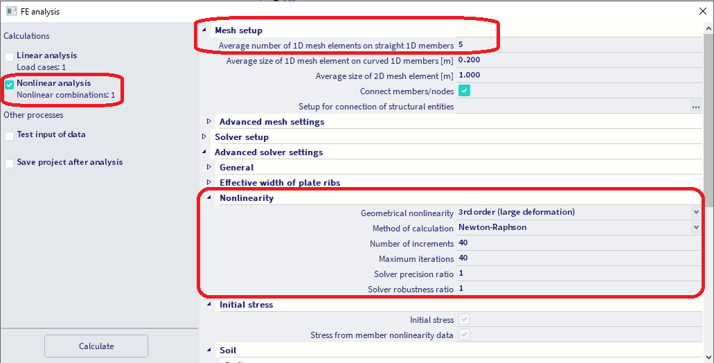
Additionally, the Solver precision ratio or Solver robustness ratio might be altered to have an influence on the convergence criteria as well.
Results
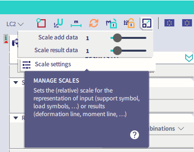
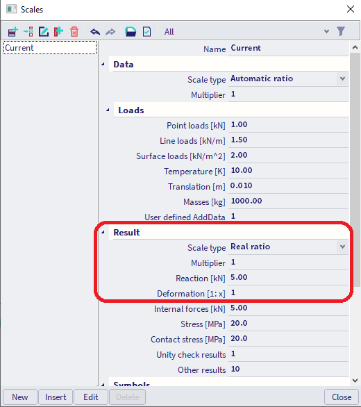
In order to see the real scale of the results (the default scale is exaggerated artificially), it is necessary to set the real ratio and the multiplier equal to 1 within the Scale setup:
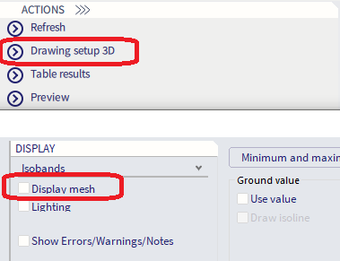
To see the 3D deformation contour plot clearly on a thin cable, the display mesh needs to be turned off within the drawing setup 3D:
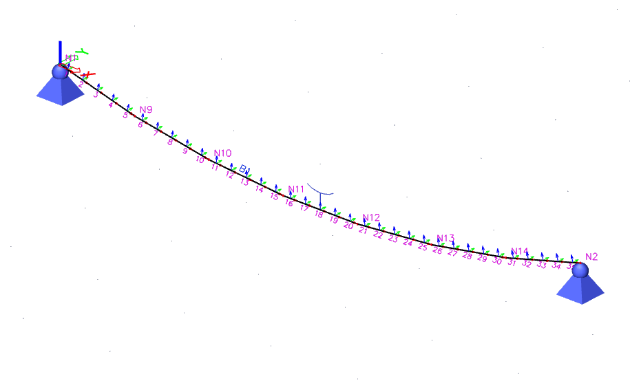
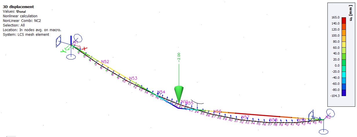
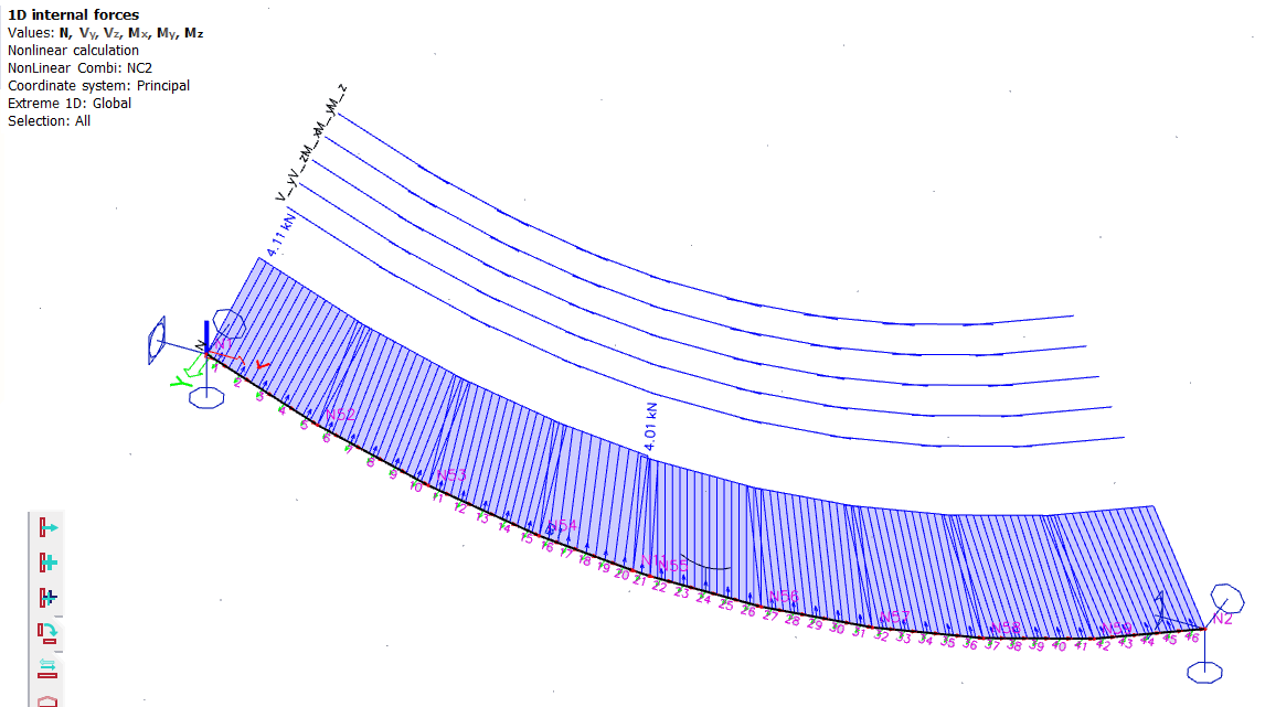
An example of a 3D displacements is depicted in the figure below:
The only non-zero values of internal forces are for normal forces N (tension):
.
Theoretical background
A curve formed by a hanging cable is called a catenary curve. With relatively small bending (height - sag roughly 10% of its length) the curve can be approximated by a parabola (this approach was implemented previously in " Design of cable members (PPE v16 and older)"). Such approximation however becomes imprecise with greater sag / length ratio (and for different heights of the begin and end nodes of the cable).
The catenary curve is linearly approximated into a poly-line. The approximation points (nodes) are calculated from the catenary equation defined by two edge points of the beam and its parameter a, which is defined as a quotient (normal force / cable weight per unit length). Normal force is defined by the user in properties and cable weight per unit length is calculated from cross section and material parameters. Formula of the general catenary equation:
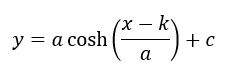
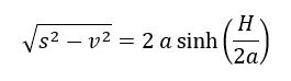
Parameters k and c represent the horizontal and vertical shifts of the curve, respectively. Computation of these parameters is thoroughly described on the web. In this web-page, the length of the catenary curve is given, in SCIA Engineer it is calculated. The relation between catenary length s, vertical span of two definition points v and their horizontal span H is:
The user has a full control of the catenary curve approximation precision. A general curvature approach has been utilized. Using the curvature (parameter defining how much the curve bends at the given point) the radius of the circles (of the same curvature as the curve in the touching point) is calculated. Concept of the approximation error is graphically described in the figure below:
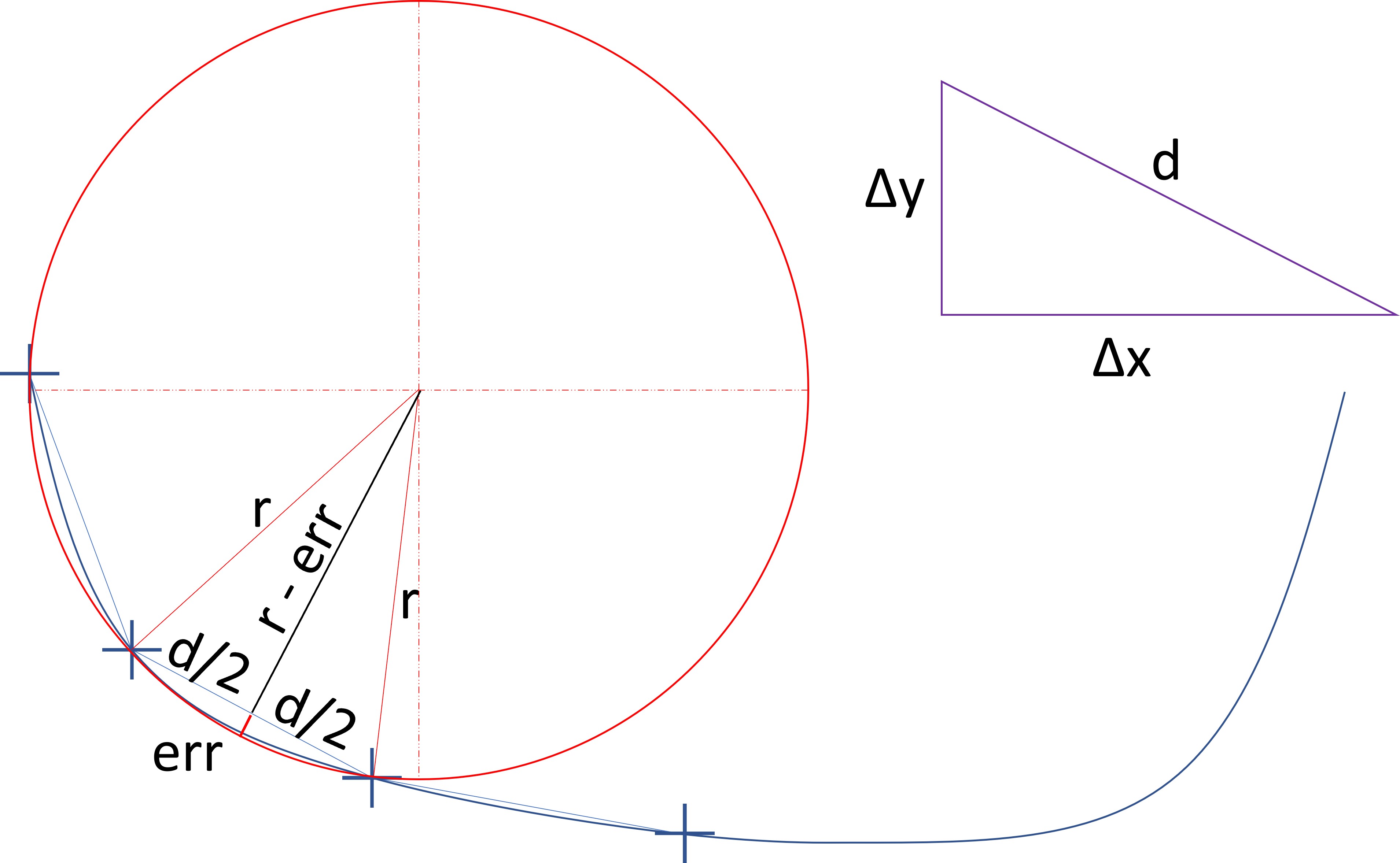
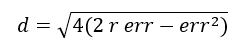
The length of the approximation line d is then:
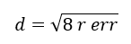
The squared err part is neglected in order to simplify the formula to:
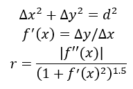
The value of the shift along x axis, Δx is obtained from the equations:
And results in a constant value of:
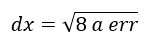
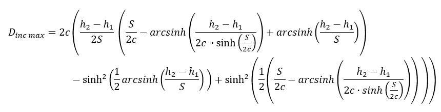
Note: It has been experimentally verified, that the maximum sag value for the approximation lines (of the curve) using this horizontal shift dx is roughly equal to err, regardless the cable length.
The value of sag (not editable in the property panel) is calculated using equation:
If some add data are connected on catenary nodes, or on any other nodes connected to catenary curve of cable (e.g. internal nodes), the relative position of these nodes remains the same on the new catenary geometry. The relative position is based on catenary curve equations, and is calculated as:
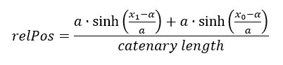
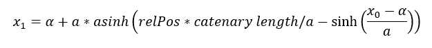
Where a is the curve parameter, x1 is the x coordinate of the given node, x0 is the x coordinate of the catenary head node and α is the shift of the curve in x-axis direction. Thex1 is then derived as:
Literature
|
1 |
|
|
2 |