Load Systems 2D

Applicable to load 2D members.

Icon of the command:

Defining of the Load system 2D

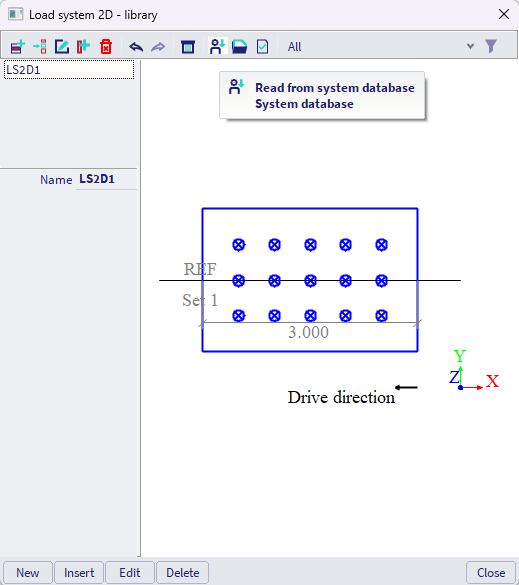
Analogically to the Load Systems 1D, in the library of the load system 2D, user can select load system either from predefined database, or create a new unique load system.

Creating new unique load system

#A -Load system might be divided into several Sets. Imagine these Sets as cars, trucks or carriages, where the distance between each set might (or does not have to) alter during the traffic.

#B1 -For each set, distributed loads might be defined by the load resultant (force, e.g. in kN), acting on an rectangular area defined by the set of 2 corner points in plane XY. Coordinates X1, Y1, X2 and Y2 of these points need to be defined. The rectangular area the surface load is applied on, is considered to be aligned with the X and Y axes of the plane XY coordinate system (hence one side of the rectangle is parallel with X and the other with Y axis; rotation of rectangle within this plane is not supported, neither different shapes as e.g. triangular area).

#B2-As the traffic load is acting on the road surface, but the central plane of the structural slab is positioned in a different height, it is possible to automatically distribute this load over larger area by defining "Load-distributing thickness" t and the "Load-distributing angle" α. The position of the corner nodes of the rectangular area the load is applied are automatically recalculated and shown as the greyed-out values next to the considered surface load.

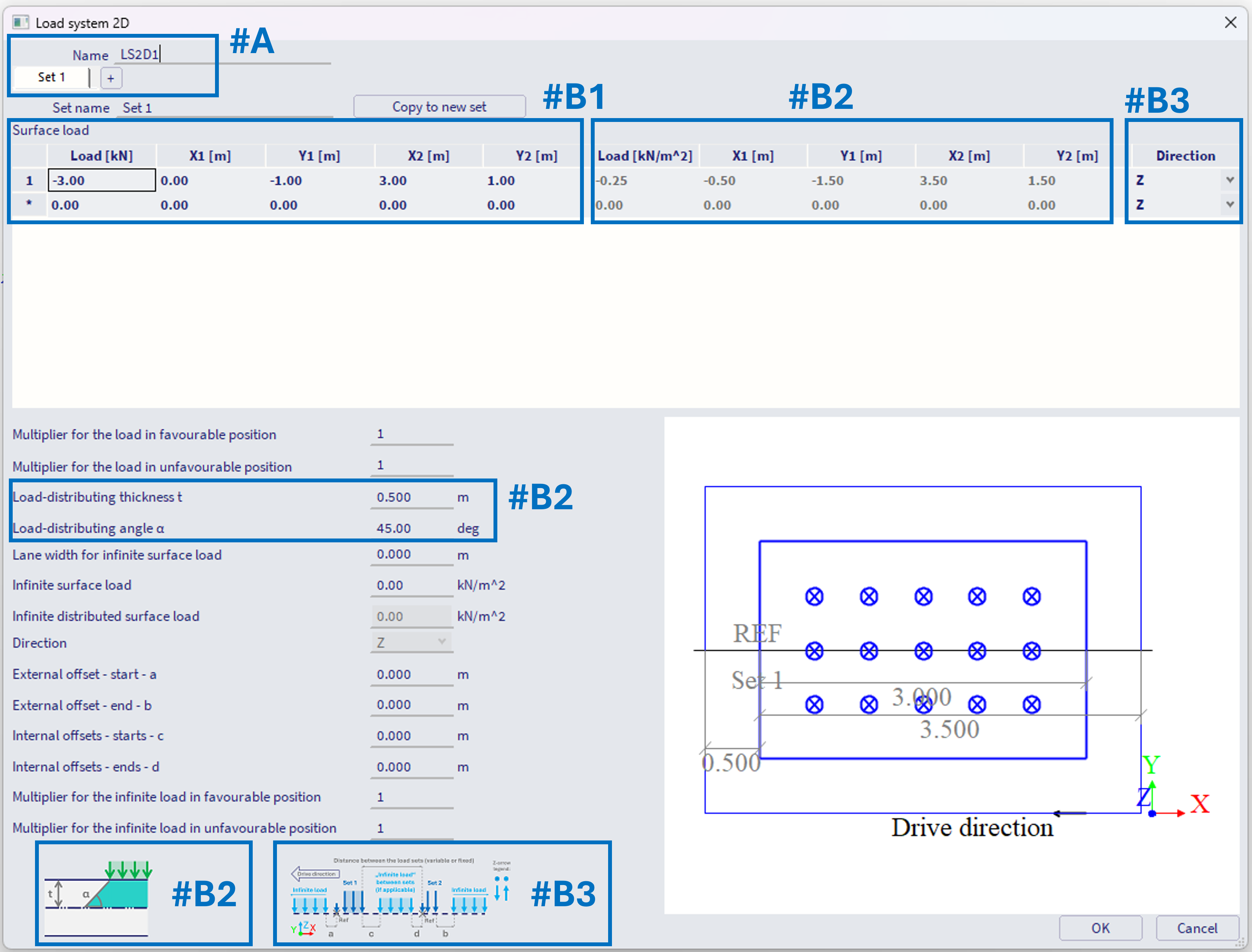
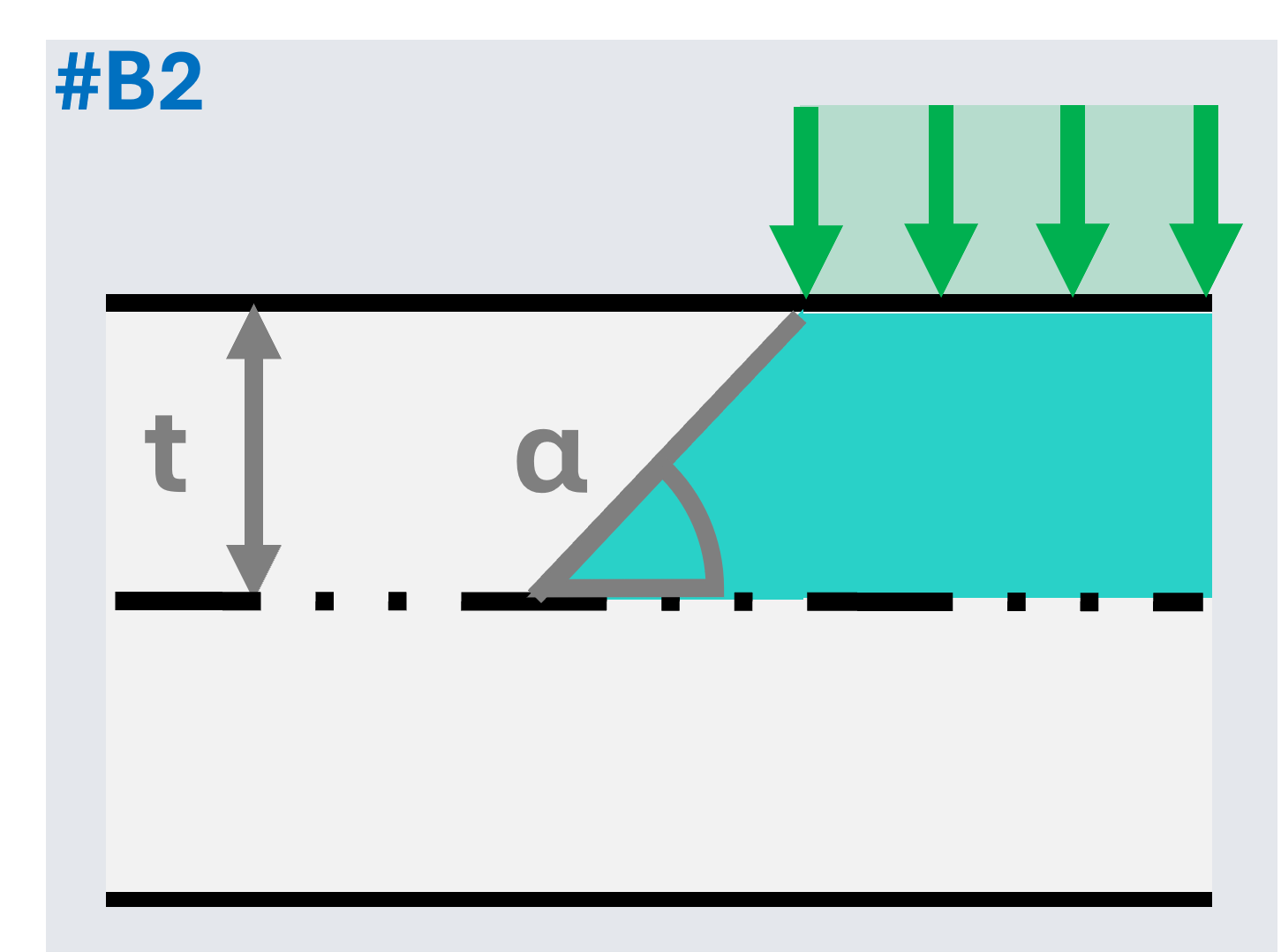
For example, in case above, the input resultant force R of -3 kN is resultant from the input rectangular area defined by points [X1,Y1], [X2,Y2], hence the defined area is 6 m^2. The load distributing angle α and the thickness t are defined in a way, that the extra offset of this area is 0.5 m. The altered coordinates of the corner points [X1',Y1'], [X2',Y2'] are considered by this algorithm:

offset = t / tan(α)

X = min(X1 , X2)

Y = min (Y1 , Y2)

length_X = abs(X2 – X1)

width_Y = abs(Y2 – Y1)

X1‘= X – offset

Y1‘= Y – offset

X2‘ = X + length_X + offset

Y2‘ = Y + width_Y + offset

so, also in case the input X1 > X2, the greyed out values will be in the order X2‘ > X1‘.

The area where the load is applied is then: A' = (length_X + 2*offset ) * (width_Y + 2*offset), in case above A' = 4 * 3 = 12 m^2

And the distributed load (greyed-out value in kN/m^2) is calculated as = R / A' ; where R is the input resultant force, hence -3 / 12 = -0.25 kN/m^2

The offset of this area is also shown in the graphical window of the defined load.

Note: User need to verify this distributed area fits within the modelled structure along whole the defined Traffic lane 2D. Any loads from areas which would be located outside the structure during the moving of the load will not be applied on the structure .

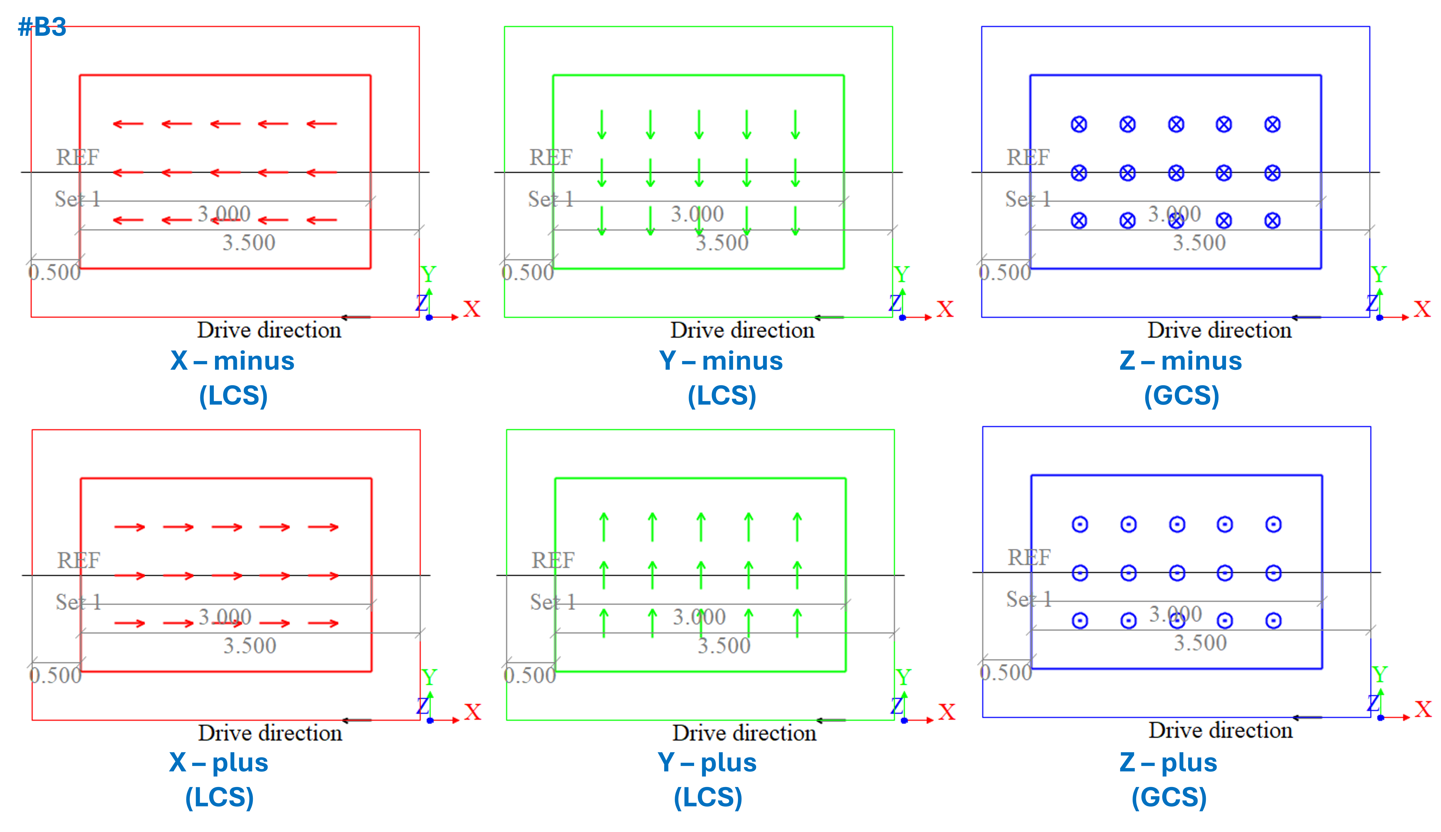
#B3-The direction of the defined load:

Z - is considered Z axis of the global coordinate system.

X or Y - are considered to be applied in local coordinate systems of the loaded slab members.

The corresponding directions of the defined loads are also plotted in the graphical window of the load system 2D. The view of this plot is from top-view, along z-axis, therefore the positive and negative signs of the z direction are distinguished by the "X" and "." symbols in the circle, resembling front and bottom view at an arrow. This is also depicted in the legend of the load system 2D, shown also in the figure below.

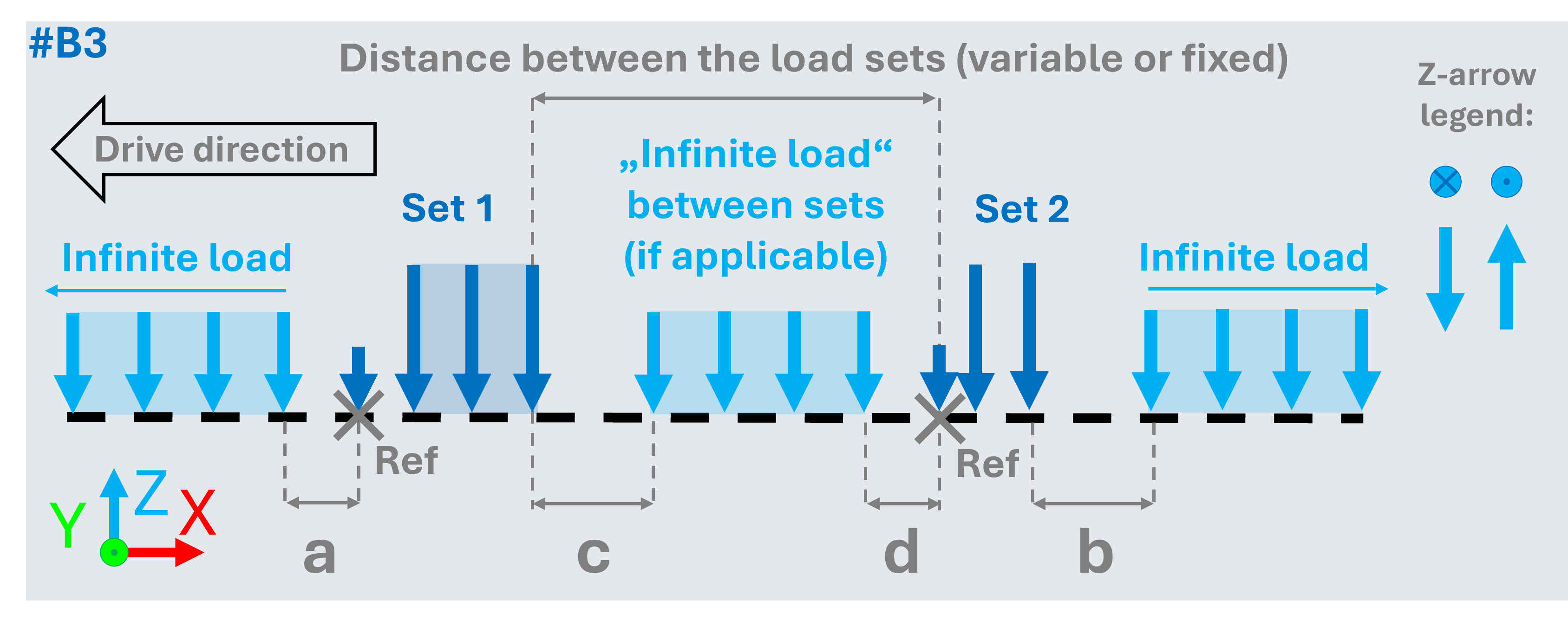
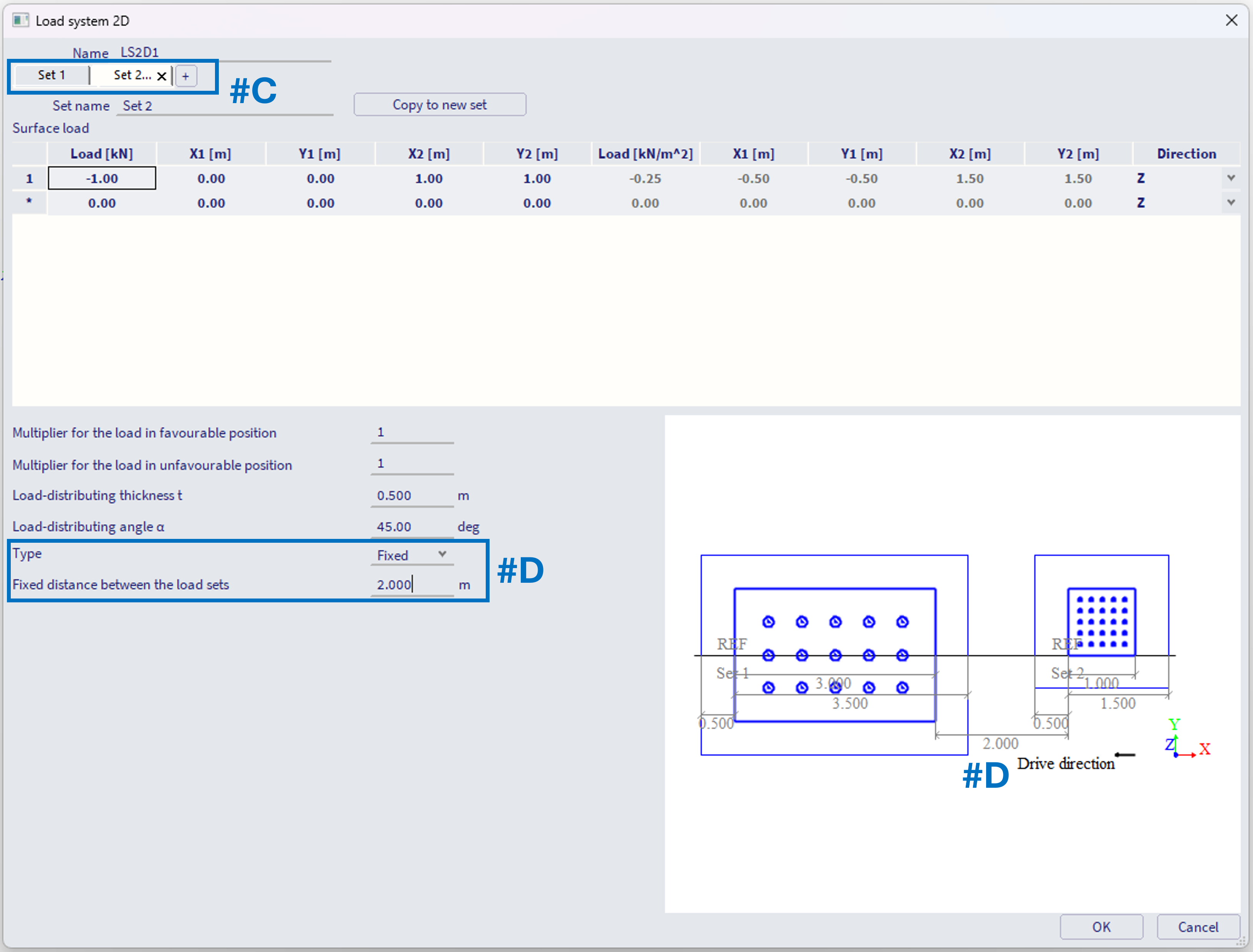
#C - Subsequent sets are created by "+" symbol in the bar, or by copying the existing set. Loads are defined the same way (steps #A, #B1, #B2, #B3). The subsequent sets are being added "backwards" from the previous set (against the drive direction, however along the positive x-axis of the plane XY which is graphically plotted)

#D - For each subsequent set (after the first set) it is necessary to define the distance from the previous set. This distance is considered from the reference point (the begin) of the current set to the position of the last load of the previous set (on example below 2 m from the end edge of the defined surface load of the set 1 to the reference point of the set 2). This distance might be defined as fixed, constant (e.g. carriages of a train not altering the mutual distance between each other).

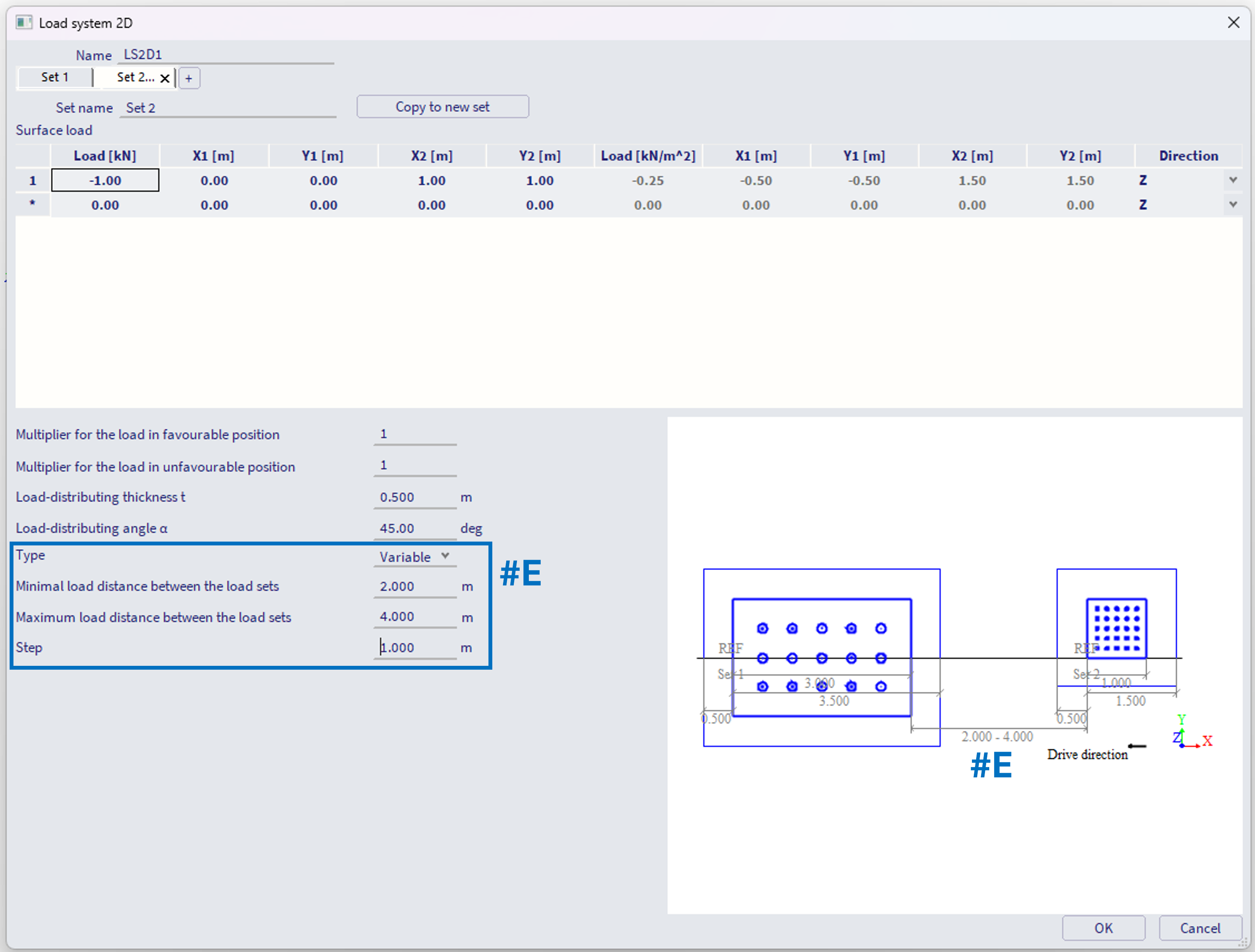
#E - Alternatively, this distance might be set as variable, with defined minimal and maximal distance between the subsequent sets, and the (maximal) step size. In example below, the minimum is 2 m, maximum 4 m with step of 1 m, what means internally three positions will be considered, distances of 2, 3 and 4 m between these sets.

Note: if the difference between the user input max and min is not divisible by the user input step without remainder, the value "(max - min) / step" is rounded up to whole number, and step size is internally considered a bit smaller, hence the step size is considered as "maximal".

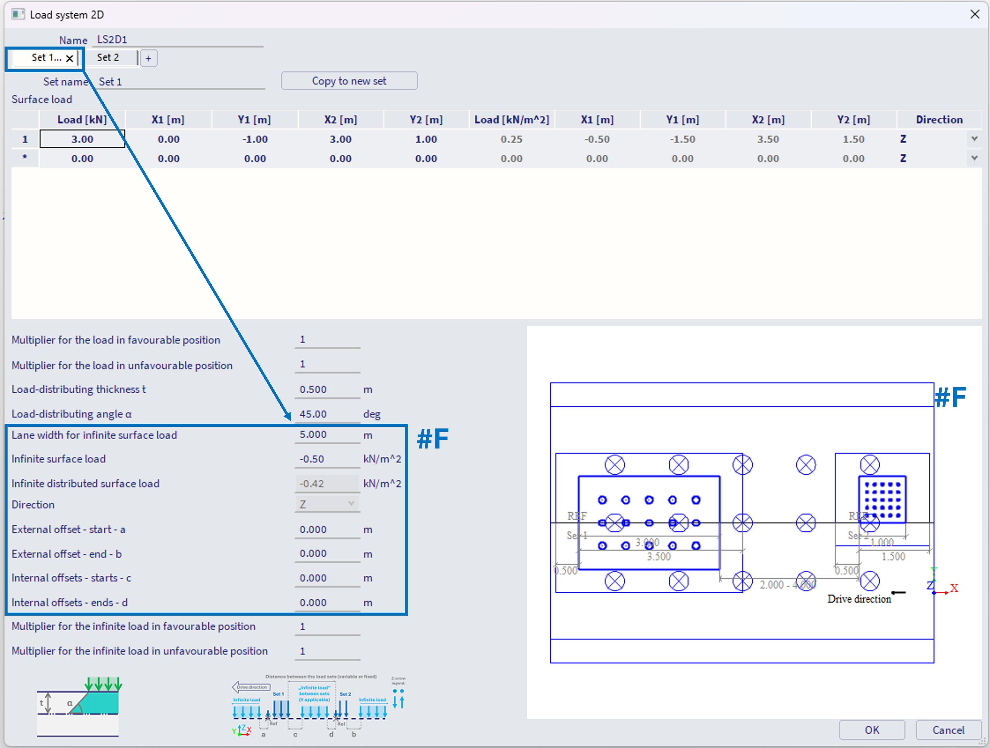
#F - It is also possible to define so called "infinite surface load".

This infinite load to be defined within the first set of the load system. It is considered (and graphically plotted in the preview) if its value is different from 0. External and internal offsets (parameters a - d) might be defined to define spacing between this infinite load and the sets of the load system.

If all these offset values a,b,c,d = 0, then the infinite load is being applied also over the load of the existing sets (see #F).

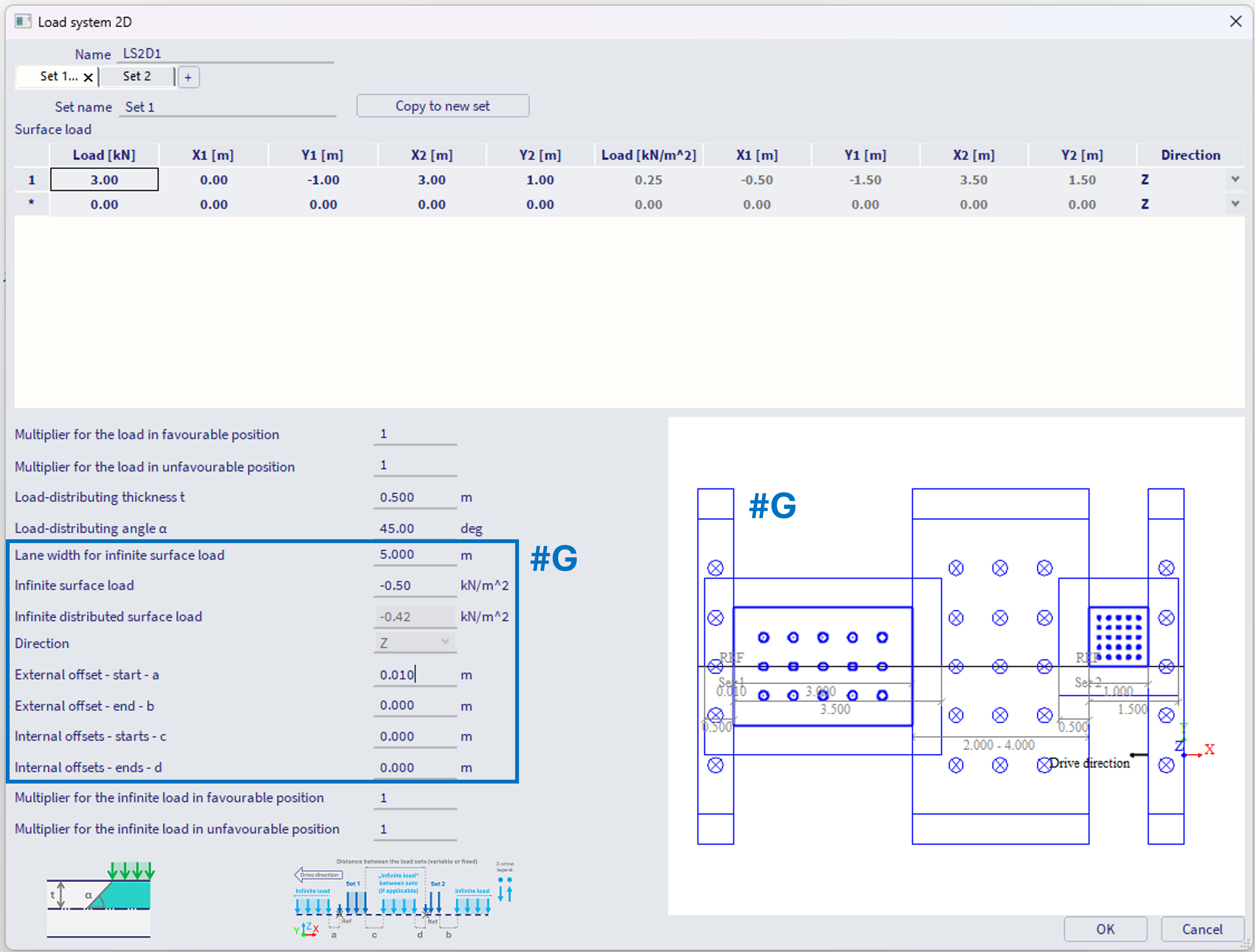
If at least one of these offset values is slightly different from 0 (e.g. a = 0.01 m), then the infinite load is being applied only between the sets, before the first set, and after the last set of the load system (see #G).

The offsets a,b,c,d are explained in the legend located directly in the load system 2D window (or also see #B3 above).

Features of the infinite load:

- The infinite load is always considered in Z axis direction (global coordinate system).

- The infinite load is considered as "infinite" along the x-axis of the traffic lane, hence along the drive direction (in the graphical plot it is depicted as along x-axis of the plane XY). Along the width of the traffic lane, the load is considered with certain finite length, definable by the parameter "Lane width for infinite surface load", in the example above this is set to 5 m. The distribution of this infinite load (feature described in #B2) is applicable, but considering only the Y direction (as this is the finite length). The load distributing angle α and the thickness t are always obtained from the first set of the load system. The input value of the infinite surface load (-0.5 kN/m^2) is then distributed on width:

Distributed width = Lane width for infinite surface load + 2 * offset (see #B2)

The greyed-out "Infinite distributed surface load" is then determined as:

Infinite distributed surface load = Infinite surface load * Lane width for infinite surface load/ Distributed width

Hence in example above: Infinite distributed surface load = -0.50 * 5 / (5+2*0.5) = -0.42 kN/m^2

- The width of the infinite load is considered evenly distributed to the both sides (right and left)

- In case the traffic lane is curved, the infinite load (and also the load from the sets) respect the curved trajectory of the traffic lane. E.g. the infinite load in curve will be split into thin rectangles, each rectangle aligned with the local tangent of the traffic lane trajectory. This will result in adding slightly more load into the inner part of the curve, and less load on the outer part. In practical purposes, where the radius of the curve is rather large, this phenomena is rather negligible. The width of these strips are based on the local mesh size of the slab elements.

Load multipliers within the Load system 2D

There are two types of multipliers for the load to be defined within sets of load system 2D. All these multipliers are ONLY considered if the load system is used within the CA entity of the Moving loads generator 2D, which is set: "Type of generated load cases = Envelope" AND the check box "Compute with Influence lines" is activated. It is being ignored in case load system is used within CA entity of the "Type of generated load cases = Envelope", where the check box "Compute with Influence lines" is off.

Alternatively, these multipliers are also considered within the CA entity of the Moving loads generator 1D, which is set: "Type of generated load cases = Influence Surfaces

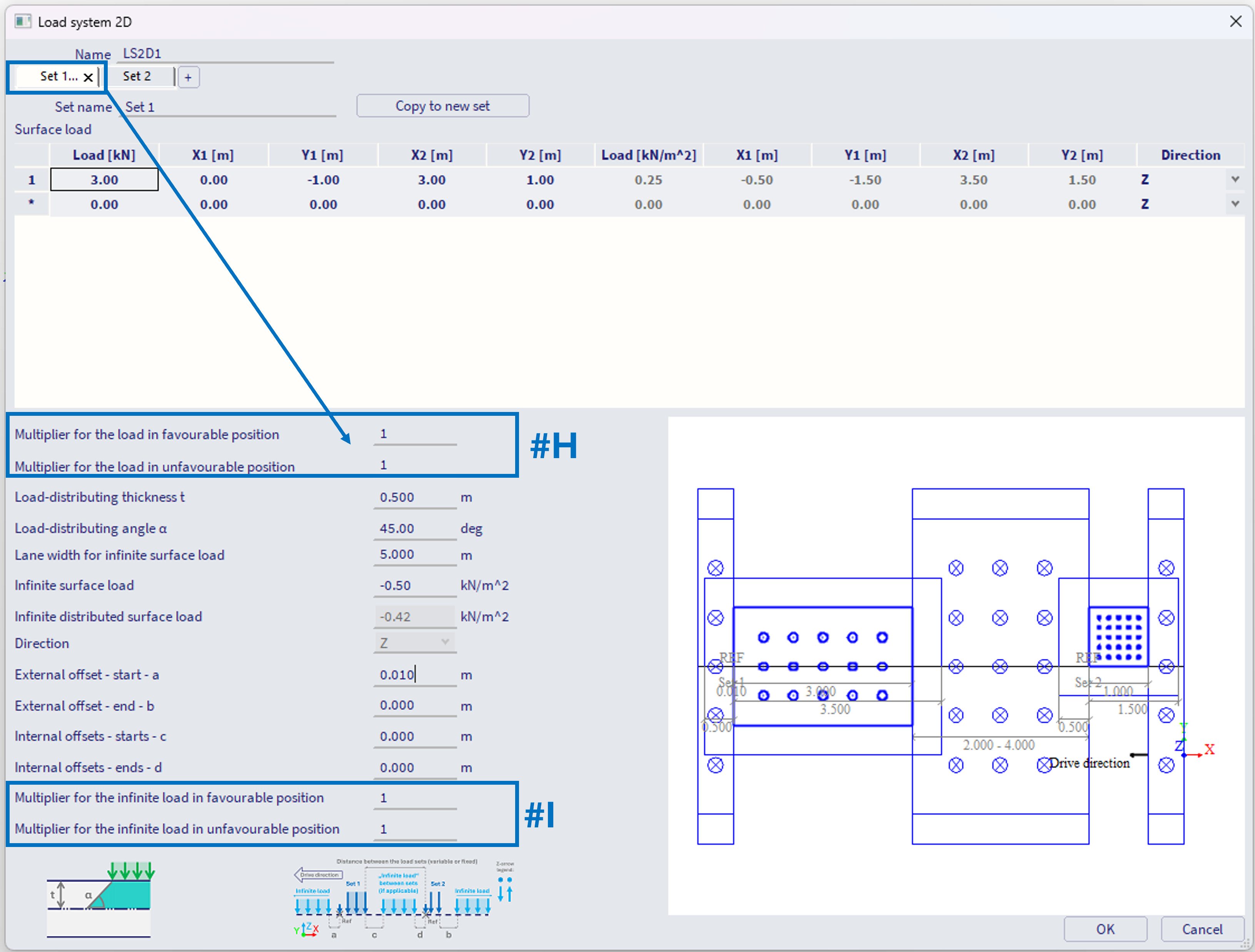
#H - Multipliers for the load:

Multiplier for the load in favourable position

Multiplier for the load in unfavourable position

These multipliers are used to multiply the load from the corresponding set, in accordance whether its current position contributes to increase or decrease of specific component (internal force) in considered position. Note: hence only usable with the influence lines option, where internally the influence lines are being calculated.

#I - Multipliers for the infinite load:

Multiplier for the infinite load in favourable position

Multiplier for the infinite load in unfavourable position

These multipliers works analogically to #H, just applied for the infinite load.

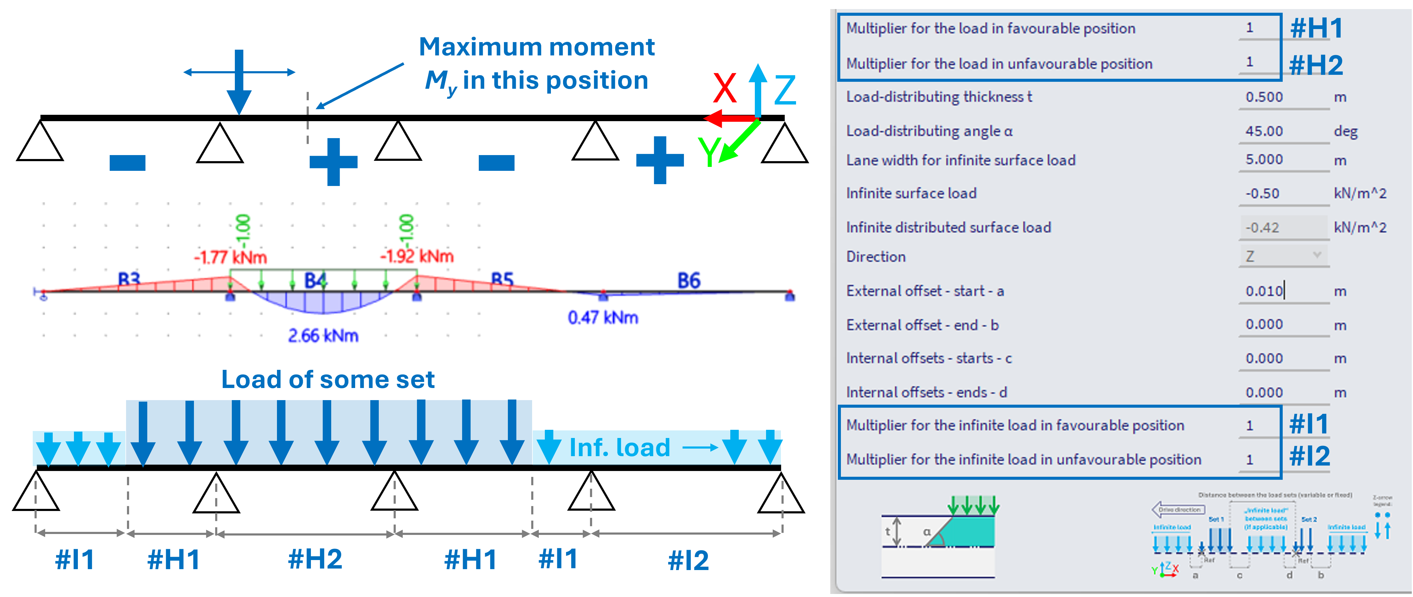
See example below (depicted on 1D beam schema, but it works analogically for 2D surfaces) - in case the extreme (positive) bending moment My is to be obtained in the middle of the second span on 4-span beam, the more load applied to 2nd and 4th span, the higher the moment. And vice versa. By setting the corresponding multipliers to 0, the load that would actually decrease the moment in this specific position is not considered at all, what would be much more conservative approach.

Notes of the features:

1) Load directions - #C - for the Z direction, the load is considered in GCS z-axis direction, for X and Y directions, the loads are considered in the LCS system of the 2D mesh elements from the slab, where the moving load is projected (based on the e Traffic lane 2D). Keep this in mind in order to consider the loads correctly.

2) The 2D solution works analogically to 1D, described in Load Systems 1D